Nora Lakhlef | Houcine Oudira* | Christophe Dumond
© 2020 IIETA. This article is published by IIETA and is licensed under the CC BY 4.0 license (http://creativecommons.org/licenses/by/4.0/).
OPEN ACCESS
The aim of this work is to show the effectiveness of a new algorithm named as modified grey wolf optimization (MGWO) algorithm to determine the optimum combination parameters values of a linear antenna array which is widely used in the communication systems. The selection part of the classical GWO has been modified by adopting the competitive exclusion selection inspired from genetic algorithm. The objective to be attained is a directional array factor with a very low level of lateral lobs. To this effect, a Gaussian function centered at 90° with the total absence of secondary lobs is considered as a desired diagram in our simulation. To matches the desired pattern as closely as possible, we considered the optimization of interspacing elements, weights amplitude and phase excitation of the linear antenna array factor. It has been demonstrated that the performance of a printed linear antenna array depends on all parameters, in which simultaneous optimization is imperative to maximize its characteristics. The obtained results show the effectiveness and the flexibility of the proposed algorithm in terms of minimized lateral lobe level compared to PSO algorithm and the convergence speed towards the desired solution.
array factor, MGWO, optimization, printed linear antenna array, synthesis
The fast increasing use of wireless communications needs an improvement in features of the network such as ability to hold, quality of service and coverage. The application of antenna array in many applications such as satellite and radar communication systems with high directivity and low side lobe level (SLL), compared to single antenna element, is an important technology that can improve the consistency and strength of a communication system [1, 2].
In this situation, the synthesis of array geometry plays a significant task in determining the physical layout of the array which generates the radiation diagram closest to the preferred one. This can be done in the case of linear array geometry through the optimization of the excitation amplitude and phase while assuming uniform spacing or while maintaining uniform excitation by the optimization of the element spacing [3, 4].
Parameters estimation to yield a preferred radiation diagram is the main task in the synthesis of pattern array. In this domain different analytical and numerical methods have been evaluated and applied to face this issue [5].
Simulated annealing (SA) [6], genetic algorithms (GA) [7] and particle swarm optimization (PSO) algorithms [8, 9] are evolutionary algorithms and successfully applied for antenna array synthesis. In this paper, a new modified grey wolf optimization has been applied to linear antenna arrays for parameters finding in the following cases: firstly, by studying the effect of each parameter optimization, then by optimizing two parameters together and finally by optimizing the whole parameters of antenna to yield a desired radiation pattern. MGWO is used to attain an array diagram with minimum side lobe level and high directivity in the specified directions. The results obtained are promising in terms of performance and efficiency.
The paper is organized as follows. Synthesis of linear antenna array and array factor equations are discussed in Section 2. Different steps of the proposed algorithm are presented in Section 3. Section 4 concerns the results and discussion. The validation of the obtained results by comparison with other optimization algorithms is also presented in this section. Finally, main conclusions are drawn in Section 5.
We consider a linear array of an identical elements along the y axis as shown in Figure 1. The corresponding array factor (AF) is given by the following equation [10]:
$\mathrm{AF}=\sum_{\mathrm{i}=1}^{\mathrm{n}} \mathrm{a}_{\mathrm{i}} \mathrm{e}^{-\mathrm{j}\left(\mathrm{ky}_{\mathrm{i}} \sin \theta-\psi_{\mathrm{i}}\right)}$ (1)
where, ai, ψi, and yi are the weight amplitude, phase of the excitation, and position of ith element in the array respectively. k is the wave number which is given by (2π/λ) and θ is the elevation angle.
$\mathrm{y}_{\mathrm{i}}=\sum_{\mathrm{p}=1}^{\mathrm{i}} \mathrm{d}_{\mathrm{i}}$ (2)
where, di is the distance between the order elements (i-1) and (i).
Figure 1. Structure of a linear array
To avoid the grating lobes appearance in one hand if large element spacing is considered [11] and the effects of mutual coupling on the other hand if the radiating elements are placed too close to each other, the following conditions must be satisfied for antenna position optimization:
$0,25 \lambda<\left|\mathrm{d}_{\mathrm{i}}\right|<2 \lambda$ (3)
The desired diagram chosen in this work is a Gaussian function which is given by:
$\mathrm{Fd}=\mathrm{n.exp}^{\frac{-\theta^{2}}{\mathrm{T}^{2}}}$ (4)
where: n is the number of radiating elements, it can be considered as the theoretical maximum gain, q is the elevation angle, and T is the standard deviation.
In this optimization procedure, a design is made to minimize the side lobe level of the radiation pattern with increasing the directivity of the main lob. To accomplish this goal, we considered the optimization of three vectors: A = [a1,a2,...,an ], ψ = [ψ1,ψ2,...,ψn] and Y = [y1,y2,...,yn] which are amplitude weights, phases excitation, and antennas position respectively using Modified Grey Wolf Optimization (MGWO) algorithm.
In this section, an optimization technique for parameters estimation of (1) is presented. To this end, we propose a new optimization technique denoted as “Modified Grey Wolf Optimization (MGWO) algorithm”. At first, we present the GWO that is introduced in 2014 by Mirjalili [12]. The philosophy of this technique, designed as optimization algorithm, inspired from searching and hunting process of grey wolves. Four types of grey wolves classified as alpha, beta, delta, and omega are employed for reproducing the mathematical model. The three major steps of hunting which are searching for prey, encircling prey and attacking prey are applied. This method belongs to meta-heuristic class since it includes many variations, and since it does not make any assumptions about the problem and can be therefore applied to a wide class of problems. Details of this algorithm are found by Mirjalili and Lewis [12] and Ali et al. [13]. The best solution is called alpha (α), the second best is beta (β), and the third best is named delta (δ). Remain candidate solutions are all considered to be omegas (ω). All of the omegas should follow the dominant types of grey wolves during the searching and hunting.
The social behavior is mathematically modeled as follow:
$\overrightarrow{\mathrm{D}}=\left|\overrightarrow{\mathrm{C}} \cdot \overrightarrow{\mathrm{X}}_{\mathrm{p}}(\mathrm{t})-\overrightarrow{\mathrm{X}}(\mathrm{t})\right|$ (5)
$\overrightarrow{\mathrm{X}}(\mathrm{t}+1)=\overrightarrow{\mathrm{X}}_{\mathrm{p}}(\mathrm{t})-\overrightarrow{\mathrm{A}} \cdot(\overrightarrow{\mathrm{D}})$ (6)
where, $t$ indicates the current iteration, $\overrightarrow{\mathrm{X}}_{\mathrm{p}}$ is the prey position vector, $\overrightarrow{\mathrm{X}}$ indicates the position vector of grey wolf, $\overrightarrow{\mathrm{A}}$ and $\overrightarrow{\mathrm{C}}$ are coefficient vectors and calculated using.:
$\overrightarrow{\mathrm{A}}=2 \overrightarrow{\mathrm{a}} \cdot \overrightarrow{\mathrm{r}}_{1}-\overrightarrow{\mathrm{a}}$ (7)
$\overrightarrow{\mathrm{C}}=2 \cdot \overrightarrow{\mathrm{r}_{2}}$ (8)
where, components of $\overrightarrow{\mathrm{a}}$ are linearly decreased from 2 to 0 over the executed iterations and $\overrightarrow{\mathrm{r}}_{1}, \overrightarrow{\mathrm{r}}_{2}$ are random numbers in [0,1]. The equations for position updating are shown as follows:
$\overrightarrow{\mathrm{D}}_{\alpha}=\left|\overrightarrow{\mathrm{C}}_{1} \cdot \overrightarrow{\mathrm{X}}_{\alpha}-\overrightarrow{\mathrm{X}}\right|$
$\overrightarrow{\mathrm{D}}_{\beta}=\left|\overrightarrow{\mathrm{C}}_{2} \cdot \overrightarrow{\mathrm{X}}_{\beta}-\overrightarrow{\mathrm{X}}\right|$
$\overrightarrow{\mathrm{D}}_{\delta}=\left|\overrightarrow{\mathrm{C}}_{3} \cdot \overrightarrow{\mathrm{X}}_{\delta}-\overrightarrow{\mathrm{X}}\right|$ (9)
$\overrightarrow{\mathrm{X}}_{1}=\overrightarrow{\mathrm{X}}_{\alpha}-\overrightarrow{\mathrm{A}}_{1} \cdot\left(\overrightarrow{\mathrm{D}}_{\alpha}\right)$
$\overrightarrow{\mathrm{X}}_{2}=\overrightarrow{\mathrm{X}}_{\beta}-\overrightarrow{\mathrm{A}}_{2} \cdot\left(\overrightarrow{\mathrm{D}}_{\beta}\right)$
$\overrightarrow{\mathrm{X}}_{3}=\overrightarrow{\mathrm{X}}_{\delta}-\overrightarrow{\mathrm{A}}_{3} \cdot\left(\overrightarrow{\mathrm{D}}_{\delta}\right)$ (10)
where, $\overrightarrow{\mathrm{X}}_{1}, \overrightarrow{\mathrm{X}}_{2}$ and $\overrightarrow{\mathrm{X}}_{3}$ represent the best three solutions so far during the iteration process, each wolf in the group update its position accordingly:
$\overrightarrow{\mathrm{X}}(\mathrm{t}+1)=\frac{\overrightarrow{\mathrm{x}}_{1}+\overrightarrow{\mathrm{X}}_{2}+\overrightarrow{\mathrm{X}}_{3}}{3}$ (11)
To solve the above optimization problem given by (1), we consider a flexible scheme using the GWO method with a slight change in the selection phase. Each search agent (position) is a vector of the parameters of optimal pattern synthesis. In this paper the proposed method is used to find specifically optimum parameters such as the weights of amplitudes, phases excitations, and inter-spacing elements that involve maintaining a directional array factor at a particular direction while simultaneously reducing the side lobe level. In the sense, the synthesized radiation pattern Fs(θ) should be as close as possible to a desired diagram Fd(θ). The fitness function to be optimize by the MGWO algorithm is given as follow:
Fitness function $=\sum_{\theta}\left(\mathrm{F}_{\mathrm{s}}(\theta)-\mathrm{F}_{\mathrm{d}}(\theta)\right)^{2}$ (12)
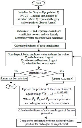
A flowchart describing the operation of the proposed scheme is shown in Figure 2. The algorithm begins by introducing the population size and maximum number of iterations. After that an initial random position is generated by using the Matlab function “rand”. To deal with the randomness of the algorithm, specific ranges limitation for the parameters finding such as the inter-elements spacing, weights amplitude and phase’s excitation are considered.
Figure 2. Flowchart of the MGWO method
The fitness function for each individual position is evaluated. Then we classify them to draw alpha, beta and delta members of the MGWO method. Accordingly, other individuals update their positions. A novel position updating concept is incorporated in the proposed scheme which provides better exploration and exploitation capability in one hand and fast convergence speed on the other hand. This new strategy is inspired from the competitive exclusion process of the genetic algorithms [14], which consists in replacing, after a comparison of the whole wolfs group positions, only the new positions of search agents (wolfs) in the current iteration that have better fitness compared to the positions fitness of the previous iterations. At the end of this phase, just the best positions of the previous and current iteration will be taken into consideration for determining the new alpha, beta and delta members, and repeats the procedure of updating the search agents’ positions according to their positions. The same process is repeated until the maximum number of iterations is reached [13-15]. The GWO with added phase has the ability to search for total optimal results without fixing any parameters as classical methods.
4.1 Comparison between MGWO and GWO
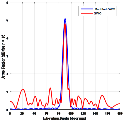
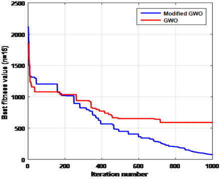
To evaluate the capabilities of the proposed method, a comparison between the MGWO and GWO to solve the design above problem is considered. In this case, the optimization of amplitudes weights, phases excitations and inter elements spacing are considered for a number of elements equal to 16.
Figure 3. Array Factor comparison as a function of elevation angle for a linear antenna array of 16 elements
Figure 4. Convergence curves for best fitness versus the number of iterations
It is clear from Figure 3 and Figure 4 that MGWO overcome the classical one in terms of achieving higher gain of the main beam while simultaneously reducing the side lobe level in one hand and providing better convergence speed on the other hand. For these reasons, in the following optimization the MGWO will be used. Table 1 confirms this remark.
Table 1. Comparative results of MGWO and GWO methods
|
|
Gain |
SSL |
HPBW |
|
MGWO |
13.8921 |
33.9835 |
5.8064 |
|
GWO |
12.8426 |
12.1343 |
5.8064 |
In the following sections, the effects of the parameters optimization such as amplitude weights, phase excitation and inter-elements spacing are considered. The optimization process is done using Matlab R2018a software in a computer with ‘Intel®Pentium®, 16 GB RAM, i7 Core processor and Windows 10 as professional operating System.
4.2 Effects of the optimized parameters on the array factor
Before studying the effect of the parameters, it has been assumed, the case without optimization, that the weights of excitation amplitude of all elements is equal to 1, their excitation phases are zero and the inter element spacing is equal to 0.5 l.
Table 2. Comparative results of each parameters effect on linear array factor
|
Number of elements |
8 |
10 |
12 |
16 |
|
|
SLL |
Without optimization |
13.0619 |
13.2288 |
13.3122 |
13.5626 |
|
Optimized spacing |
16.4640 |
18.1226 |
19.3534 |
19.7471 |
|
|
Optimized amplitude |
14.4796 |
17.2519 |
18.1274 |
19.7325 |
|
|
Optimized phase |
13.0204 |
13.1586 |
13.4348 |
13.4348 |
|
|
HPBW |
Without optimization |
13.0645 |
10.2822 |
8.7097 |
6.5322 |
|
Optimized spacing |
11.3365 |
9.9540 |
8.2258 |
5.6854 |
|
|
Optimized amplitude |
12.9953 |
11.0600 |
9.6775 |
7.4655 |
|
|
Optimized phase |
12.7188 |
9.6775 |
8.2950 |
6.0830 |
|
Table 3. Comparative results of two parameters effect on linear array
|
Number of elements |
8 |
10 |
12 |
16 |
|
|
SLL |
Without optimization |
13.0619 |
13.2288 |
13.3122 |
13.5626 |
|
Optimized spacing & phase |
16.4737 |
17.3025 |
19.6508 |
21.0321 |
|
|
Optimized amplitude & spacing |
17.3541 |
20.1556 |
23.5185 |
25.0379 |
|
|
Optimized amplitude & phase |
15.2091 |
17.5438 |
20.7539 |
24.5477 |
|
|
HPBW |
Without optimization |
13.0645 |
10.2822 |
8.7097 |
6.5322 |
|
Optimized spacing & phase |
11.0600 |
9.4010 |
8.5715 |
6.0830 |
|
|
Optimized amplitude & spacing |
9.9540 |
9.1245 |
8.2950 |
7.4655 |
|
|
Optimized amplitude & phase |
13.2718 |
11.0600 |
9.9540 |
7.4655 |
|
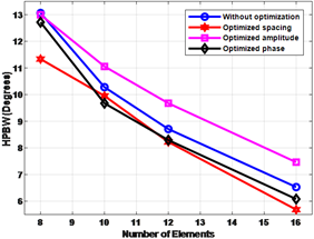
4.2.1 Influence of each parameter on the array factor
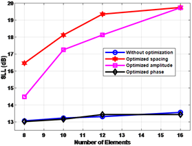
In this experiment, the effect of each parameter optimization such as amplitude weights, phase excitation and inter-elements spacing on the array factor is considered. To this end, it has been assumed the optimization of one parameter while keeping constant the remaining ones, which leads to a one degree of freedom. By investigating the illustrated results (Table 2), it is observed that an appropriate inter-element spacing can change the overall array pattern and allows the designer to have more control over the array pattern in terms of directivity and reduced SLL.
From the Figure 5, it can be noticed also that, the inter-element spacing has a large influence compared to the others in terms of reducing SLL while the effect of the phase is negligible. When the half power beam width (HPBW) is considered (Figure 6), the influence of excitation phase is significant and the inter-elements spacing effect is still more powerful than the others in most case.
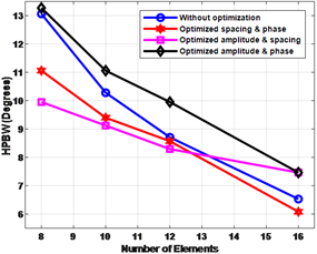
4.2.2 Influence of two parameters together on the array factor
In this case, the optimization of two parameters is considered, which leads to two degrees of freedom, Phase-spacing, amplitude-spacing and phase-amplitude (Table 3). A closed look to the reported results demonstrates that, by optimizing both amplitude and spacing, we get better results in terms of reaching the main lobe in the preferred direction with minimal SLL in almost cases (Figures 7 and 8). From this case, we note that the optimization of the amplitude and spacing together provides the best result in terms of reduce SLL then the amplitude and phase and finally the spacing and phase.
4.2.3 Effects of all parameters on the array factor
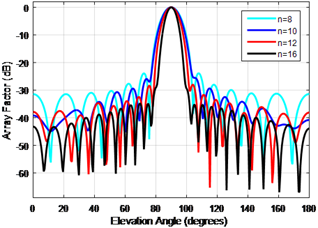
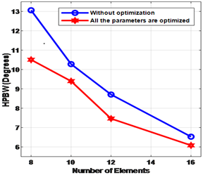
In the last case, we have considered the optimization of the inter-element spacing, weights amplitude and phase excitation together. In this case, all the unknown parameters are estimated and the corresponding array factors are illustrated by the Figure 9 which is normalized with respect to the maximum value of the main lobe. From this figure, for N =8, 10, 12 and 16 elements respectively, when all parameters are optimized, the HPBW improves and SLL reduced with the increase of the number of elements. It can be also noticed that this case provides better performance compared to the cases when two parameters and/or one parameter are controlled.
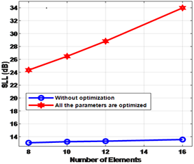
The numerical values of the corresponding SLL and HPBW are grouped in Table 4 that validates this remark. From the Figure 10 and 11, it can be noticed also that, as the number of elements increase the SLL degrease while its effect on HPBW is not significant.
Figure 5. SLL as a function of elements number
Figure 6. HPBW as a function of elements number
Table 4. Comparative results of parameters optimization for linear antenna array
|
Number of elements |
8 |
10 |
12 |
16 |
|
|
SLL |
Without optimization |
13.0619 |
13.2288 |
13.3122 |
13.5626 |
|
All the parameters are optimized |
24.3397 |
26.4751 |
28.8200 |
33.9835 |
|
|
HPBW |
Without optimization |
13.0645 |
10.2822 |
8.7097 |
6.5322 |
|
All the parameters are optimized |
10.5070 |
09.4000 |
7.4654 |
6.0830 |
|
Figure 7. SLL as a function of elements number
Figure 8. HPBW as a function of elements number
Figure 9. Variation in Array Factor as a function of elevation angle when all the parameters are optimized for different values of n
Figure 10. SLL as a function of elements number
Figure 11. HPBW as a function of elements number
4.3 Comparison with literature
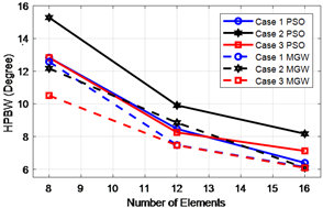
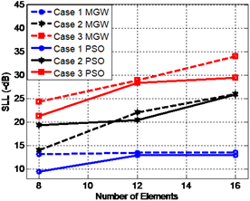
In this part, the obtained results are compared with the reference [9]. For the seek of an objective comparison; we study the same cases which are presented in the cited reference. In case 1: the phase excitation has been optimized, while the weights amplitude have been considered uniform and equal to 1 and the inter-element spacing are fixed to 0.5 l, Case 2: excitation of weights amplitudes and phases excitation have been optimized while the inter-element spacing are kept constant (0.5 l), Case 3: the three parameters have been optimized simultaneously. Figure 12 shows the HPBW for the cases discussed above. A closer look to this figure confirms that a considerable improvement in HPBW when we have more control parameters. We can notice also that by controlling inter-element spacing, a significant improvement in the antenna array characteristics is observed. Figure 13 illustrates the corresponding results for SLL when considering the same cases. The figure shows that SLL reduces considerably as we move from Case 1 to 3, i.e., results corresponding to Case 3 are better than Case 2 and 1.
In summary, from the obtained results, the optimized parameters using modified grey wolf optimization method provide better performance compared to the results obtained by particle swarm optimization algorithm [9] in most cases.
Figure 12. HPBW as a function of elements number
Figure 13. Side Lobe Level as a function of elements number
In this work, a new proposed algorithm denoted as MGWO for the synthesis and optimization of a linear antenna array is applied. The array factor is used to evaluate its characteristics such as the width of the half-beam width, and the Side Lobe Level. The proposed algorithm is tested on each parameter, two parameters together and then on the three parameters simultaneously. It has been demonstrated that the performance of a printed linear antenna array depends on all parameters, in which simultaneous optimization of the inter-elements spacing and weights of complex currents is imperative to maximize its characteristics. For linear antenna array of 16 elements, it can be noticed that – 33.9835dB SLL has been obtained when MGWO algorithm is used whereas –12.1443dB and -29.4316dB obtained by using traditional GWO and PSO optimization algorithms respectively. There is a significant reduction of SLL of – 4.5519dB and -21.8392 dB when compared to GWO and PSO optimized algorithms.
By investigating the obtained results, it is observed that the optimization of linear antenna arrays using MGWO provides considerable enhancements compared to the synthesis obtained from the GWO and PSO algorithm. The results suggest that the effectiveness of the proposed scheme will be more useful in wireless systems for noise free communication when the optimization complexity increases.
[1] Carver, K.R., Mink, J.W. (1981). Microstrip antenna technology. IEEE Trans. Antennas and Propagation, 29(1): 2-24. http://dx.doi.org/10.1109/TAP.1981.1142523
[2] Howell, J.Q. (1975). Microstrip antennas. IEEE. Transactions on Antennas and Propagation, 23(1): 90-93. https://dx.doi.org/10.1109/TAP.1975.1141009
[3] Chen, T.B., Chen, Y.B., Jiao, Y.C., Zhang, F.S. (2005). Synthesis of antenna array using particle swarm optimization. 2005 Asia-Pacific Microwave Conference Proceedings, Suzhou, China. https://dx.doi.org/10.1109/APMC.2005.1606685
[4] Recioui, A., Azrar, A., Bentarzi, H., Dehmas, M., Chalal, M. (2008). Synthesis of linear arrays with side lobe reduction constraint using genetic algorithm. International, Journal of Microwave and Optical Technology, 3(5): 524-530.
[5] Unz, H. (1960). Linear arrays with arbitrarily distributed elements. IEEE Transactions on Antennas and Propagation, 8(2): 222-223. https://dx.doi.org/10.1109/TAP.1960.1144829
[6] Lee, K.C. (2005). Frequency-domain analyses of nonlinearly loaded antenna arrays using simulated annealing algorithms. Progress in Electromagnetics Research, 53: 271-281. https://dx.doi.org/10.2528/PIER04101501
[7] Raniszewski, A. (2016). Radiation pattern synthesis for RADAR application using Genetic Algorithm. 21st International Conference on Microwave Radar and Wireless Communications, Krakow, Poland. http://dx.doi.org/10.1109/MIKON.2016.7492086
[8] Panduro, M.A., Brizuela, C.A., Balderas, L.I., Acosta, D.A. (2009). A comparison of genetic algorithms, particle swarm optimization and the differential evolution method for the design of scannable circular antenna arrays. Progress in Electromagnetics Research B, 13: 171-186. https://dx.doi.org/10.2528/PIERB09011308
[9] Saleem, S.S., Ahmed, M.M., Rafique, U., Ahmed, U.F. (2016). Optimization of linear antenna array for low SLL and high directivity. 2016 19th International Multi-Topic Conference (INMIC), Islamabad, Pakistan. http://dx.doi.org/10.1109/INMIC.2016.7840132
[10] Balanis, C.A. (2003). Antenna Theory: Analysis and Design. (2 ed edition). Singapore, John Wiley & Sons.
[11] Kildal, P.S., Vosoogh, A., Maci, S. (2015). Fundamental directivity limitations of dense array antennas: A numerical study using Hannan’s embedded element efficiency. IEEE Antennas and Wireless Propagation Letters, 15: 766-769. https://dx.doi.org/10.1109/LAWP.2015.2473136
[12] Mirjalili, S.M., Lewis, A. (2014). Grey wolf optimizer. Advances in Engineering Software, 69: 46-61. https://doi.org/10.1016/j.advengsoft.2013.12.007
[13] Ali, M., El-Hameed, M.A., Farahat, M.A. (2017). Effective parameters’ identification for polymer electrolyte membrane fuel cell models using grey wolf optimizer. Renewable Energy, 111(c): 455-462. https://doi.org/10.1016/j.renene.2017.04.036
[14] Herrer, F., Lozano, M., Verdegay, J.L. (1998). Tackling real-coded Genetic algorithms: Operators and tools for behavior al analysis. Artificial Intelligence Review, 12: 265-319. https://doi.org/10.1023/A:1006504901164
[15] Hatta, N.M., Zain, A.M., Sallehuddin, R., Shayfull, Z., Yusoff, Y. (2019). Recent studies on optimisation method of Grey Wolf Optimiser (GWO): A review (2014–2017). Artificial Intelligence Review, 52: 2651-2683. https://doi.org/10.1007/s10462-018-9634-2