Raja Ram Yadav* | Joy Roy
OPEN ACCESS
In present study, solution of advection-dispersion equation is obtained to determine concentration distribution of solute introduced from a varying pulse type point source in one-dimensional heterogeneous semi-infinite porous medium. Heterogeneity of the medium gives rise to space dependent groundwater velocity, dispersion coefficient and retardation factor. Groundwater velocity is some exponent ξ to a linear function of space. The dispersion and retardation factor are also exponents of same linear function with exponents (ξ+1) and (ξ-1), respectively, where ξ takes the value 0 or 1. At one end of the domain, a time dependent varying nature source, which involves step-size increasing function of time, acts along the flow up to a certain time the n eliminated while concentration gradient is considered zero at the other end of the domain. Initially, medium is uniformly polluted. Firstly, the advection-dispersion equation is reduced into constant coefficients by using certain transformations and then Laplace Integral Transformation Technique is utilized to get the solution. The obtained result is illustrated with numerical examples to study the effect of various parameters.
advection, dispersion, aquifer, porous medium, Laplace transformation technique
The movement of solutes through porous formation has earned great importance in the application of soil physics, groundwater hydrology and many others. Nowadays, groundwater pollution has become major concern of scientist working in the area of hydrology, soil physics, environmental engineering and mathematics. Mathematical models are the very effective and reliable tools for predicting water quality and assessing the affected area. Hydraulic conductivity and porosity are the key features influencing the solute transport along groundwater flow. Temporal variation in hydraulic gradient causes the temporal variation in velocity. These parameters depend on the size i.e., the volume of the aquifer and are usually used to calculate average linear velocity. Over last few decades there have been several research articles (analytical and numerical both) developed for predicting the conservative solute transport in groundwater. Analytical solutions of one-dimensional solute transport problems in finite and semi-infinite domain subject to various initial and boundary conditions have been published in literature [1-5]. Serrano [6] studied the effect of recharge and physical hydrologic variables on the solute dispersion parameters in one-dimensional aquifers. The literature [7] derived analytical solution for one-dimensional solute transport with scale dependent exponentially increasing dispersion coefficient under time varying boundary condition. Dagan [8] analyzed the scale-dependent dispersion under variable decay and retardation factor. One-dimensional solute transport with linear asymptotic scale dependent dispersion discussed in the paper [9]. It’s observed that temporally dependent dispersity is an arbitrary function of time [10, 11]. Heterogeneity was considered as major feature of solute transport in aquifer [12-14]. The authors [15-17] obtained the analytical solution for advection dispersion equation with linear and quadratic spatial/temporal coefficients using LITT and GITT. Belyaev et al. [18] obtained analytical and numerical solutions with spatially dependent dispersion in heterogeneous aquifer. Analytical solution was derived for one-dimensional advection-dispersion equation with asymptotic dispersivity [19]. You and Zhan [20] evaluated analytical solution for one-dimensional solute transport with time-dependent sources and exponential spatial type dispersivity. Sanskrityayn et al. [21] established an analytical solution for one-dimensional advection-dispersion equation using Green function method for instantaneous and continuous point source along with mutually proportional dispersion and velocity in groundwater and river in system.
The aim of this paper is to extend the study in the paper [22] by taking varying nature pulse type input by involving step-size time function. This aim is based upon the fact that solute introduction to water bodies which is profusely governed by varying nature input rather than uniform nature was due to presence of natural phenomena and manmade activities [23]. In this theoretical model, groundwater velocity, dispersion coefficient and retardation factor depend on some exponent of linear space function because of heterogeneity of the medium and concentration distribution is assumed to be uniform at beginning of study. The Laplace Integral Transform Technique (LITT) is applied to get the solution. Such solution may prove much effective in dealing a real life solute transport related problems.
The solute movement through porous medium is the result of two phenomena advection and dispersion which is combined effect of mechanical mixing and molecular diffusion. The second order parabolic equation, which includes all these factors, is called advection-dispersion equation. This equation obtained by using Darcy’s law, the principle of mass conservation and Fick’s laws of diffusion is given as [24]:
$R(x, t) \frac{\partial c}{\partial t}=\frac{\partial}{\partial x}\left(D(x, t) \frac{\partial c}{\partial x}-u(x, t) c\right)$ (1)
where, c[ML-3] is the solute concentration of the pollutant transporting along the flow field through the medium at a position x[L] and time t[T]. D[L2T-1] and u[LT-1] are the longitudinal dispersion and groundwater velocity, respectively. R is retardation factor which is a dimensionless quantity. The term on the left hand side of the Eq. (1) accounts for change in concentration with time in liquid phase. The first and second terms on the right-hand side of the Eq. (1) represent the influence of the dispersion on the concentration distribution and change of concentration due to advective transport in longitudinal direction, respectively.
In reality, velocity and dispersion coefficients in the aquifer are variable due to change in hydraulic gradient. Freeze and Cherry [25] asserted that coefficient of dispersion is proportional to some exponent of groundwater velocity and exponent may lie within the range [1, 2], i.e., $D \propto u^{\psi}$ and $1 \leq \psi \leq 2$.
The coefficient of dispersion is considered directly and squarely to proportional to groundwater velocity [26, 27].
According to the literature [28], dispersivity, which is ratio of dispersion and groundwater velocity may be linear, quadratic, exponential, and asymptotic. Chatterjee and Singh [29] proposed two-dimensional solution by stating that besides zero velocity along the depth dispersion may not vanish in same direction.
In this article, let the groundwater velocity and Dispersion coefficient be some exponent of linear function of space as: $u(x, t)=u_{0}(1+a x)^{\xi}$, $D(x, t)=D_{0}(1+a x)^{\xi+1}$, where heterogeneity factor a is a non-zero real constant having dimension that is inverse of space variable and is accounting for the variations in velocity and dispersion due to heterogeneity and ξ, a dimensionless parameter, sets a respective spatial relation between dispersion, groundwater velocity. Yadav and Kumar [30] assumed retardation as exponentially decreasing function of space. In present study retardation factor is assumed as function of space $R(x, t)=R_{0}(1+a x)^{\xi-1}$. Let 0 <ax ≤ 1 to keep the value in order. Different values of a will represent different heterogeneity nature. Therefore, Eq. (1) may be re-written as:
$R_{0}(1+a x)^{\xi-1} \frac{\partial c}{\partial t}=\frac{\partial}{\partial x}\left(D_{0}(1+a x)^{\xi+1} \frac{\partial c}{\partial x}-u_{0}(1+a x)^{\xi} c\right)$ (2)
The Eq. (2) takes the advection-dispersion equation of the papers [31] and [14] for ξ=1 and ξ=-1, respectively. In present paper we have considered that ξ can take the values for ξ=0 and ξ=1. When ξ=0, the groundwater velocity is constant while dispersion is linear function of space and retardation factor is inversely proportional to linear function of space. For ξ=1, dispersion is squarely proportional to groundwater velocity which is linear function of space and retardation factor is reduced to a constant. Initially, concentration distribution is taken uniform throughout the domain and is represented by following condition Eq. (3). Input source of varying nature is defined mathematically by following Eqns. (4a, b) or (5a, b). The Eq. (6) refers that concentration gradient is equal to zero at other end of the domain. Mathematically, initial and boundary conditions for proposed problem may be written as:
$c(x, t)=c_{i} ; t=0 x \geq 0$ (3)
$\left\{\begin{array}{l}-D(x, t) \frac{\partial c}{\partial x} \\ +u(x, t) c\end{array}\right\}=\left\{\begin{array}{l}u_{0}\left(c_{0}+\alpha\left[\frac{t}{n}\right]\right) ; 0<t \leq t_{0} \\ x=0 \\ 0 ; t>0\end{array}\right.$ (4a-4b)
Or
$\left\{\begin{array}{l}-D_{0}(1+a x)^{\xi+1} \times \\ \frac{\partial c}{\partial x}+u_{0}(1+a x)^{\xi} c\end{array}\right\}=\left\{\begin{array}{l}u_{0}\left(c_{0}+\alpha\left[\frac{t}{n}\right]\right) ; 0<t \leq t_{0} \\ x=0 \\ 0 ; t>0\end{array}\right.$ (5a-5b)
$\frac{\partial c(x, t)}{\partial x}=0, x \rightarrow \infty, t \geq 0$ (6)
where, [] represents least integer function. a[ML-3] is a parameter which regulates the step-size increment in input concentration or extra flow in per n years over the previous n year’s slot within the time less than or equal to t0. In present study, n is taken a positive integer.
Now introducing a new space variable, X with the transformation as:
$X=\frac{1}{a} \log (1+a x)$ or $x=\frac{1}{a}\{\exp (a X)-1\}$ (7)
It is obvious that X=0 at x=0 and X>0 when x>0.
Using transformation in Eq. (7), Eqns. (2)-(6) may be written as:
$R_{0} \frac{\partial c}{\partial t}=D_{0} \frac{\partial^{2} c}{\partial X^{2}}-\left(u_{0}-D_{0} \xi a\right) \frac{\partial c}{\partial X}-u_{0} \xi a c$
Or,
$R_{0} \frac{\partial c}{\partial t}=D_{0} \frac{\partial^{2} c}{\partial X^{2}}-w_{0} \frac{\partial c}{\partial X}-\mu_{1} c$ (8)
where, $w_{0}=u_{0}-D_{0} \xi a$ and $u_{1}=u_{0} \xi a$
$c(X, t)=c_{i} ; t=0, X>0$ (9)
$\left\{\begin{array}{l}-D_{0} e^{\xi a X} \times \\ \frac{\partial c}{\partial X}+u_{0} e^{\xi a X} c\end{array}\right\}=\left\{\begin{array}{l}u_{0}\left(c_{0}+\alpha\left[\frac{t}{n}\right]\right) ; 0<t \leq t_{0} \\ X=0 \\ 0 ; t>0\end{array}\right.$ (10a-10b)
$\frac{\partial c(X, t)}{\partial X}=0 ; X \rightarrow \infty, t \geq 0$ (11)
In order to remove convective term from Eq. (8), we apply following transformation:
$c(X, t)=k(X, t) \exp \left[\frac{w_{0}}{2 D_{0}} X-\frac{1}{R_{0}}\left(\frac{w_{0}^{2}}{4 D_{0}}+\mu_{1}\right) t\right]$ (12)
where, k(X, t) is a new dependent variable depending on space and time.
Using transformation in Eq. (12), the Eqns. (8)-(11) may be written as:
$R_{0} \frac{\partial k}{\partial t}=D_{0} \frac{\partial^{2} k}{\partial X^{2}}$ (13)
$k(X, t)=c_{i} \exp (-\beta X) ; t=0, X>0$ (14)
$\left\{\begin{array}{l}-D_{0} e^{\xi a X} \frac{\partial k}{\partial X}+ \\ \left(u_{0}-\frac{w_{0}}{2}\right) e^{\xi a X} k\end{array}\right\}==\left\{\begin{array}{l}\left(\begin{array}{l}u_{0}\left(c_{0}+\alpha\left[\frac{t}{n}\right]\right) \\ \times \exp \left(\eta^{2} t\right)\end{array}\right\} ; 0<t \leq t_{0} \\ X=0 \\ 0 ; t>0\end{array}\right.$ (15a-15b)
$\frac{\partial k(X, t)}{\partial X}+\frac{w_{0}}{2 D_{0}} k(X, t)=0 ; X \rightarrow \infty, t>0$ (16)
where,
$\beta=\frac{w_{0}}{2 D_{0}}$ and $\eta=\sqrt{\frac{1}{R_{0}}\left(\frac{w_{0}^{2}}{4 D_{0}}+\mu_{1}\right)}=\frac{\left(u_{0}+D_{0} a \xi\right)}{2 \sqrt{R_{0} D_{0}}}$ (17)
Applying Laplace Transformation to Eqns. (13)-(16), the boundary value problem reduced into an ordinary differential equation of second order, which includes following three equations.
$\frac{d^{2} \bar{k}}{d X^{2}}-\frac{p R_{0}}{D_{0}} \bar{k}=-\frac{R_{0}}{D_{0}}\left[c_{i} \exp (-\beta X)\right]$ (18)
$-D_{0} \frac{d \bar{k}}{d X}+\left(u_{0}-\frac{w_{0}}{2}\right) \bar{k}=u_{0} c_{0} \frac{\left[1-\exp \left\{-\left(p-\eta^{2}\right) t_{0}\right\}\right]}{\left(p-\eta^{2}\right)}+$
$\sum_{r=0}^{T-1} u_{0} \alpha(r+1) \frac{\exp (-p n r)}{\left(p-\eta^{2}\right)} \exp \left(\eta^{2} n r\right)-\sum_{r=0}^{T-1} u_{0} \alpha(r+1) \times$
$\frac{\exp \{-p n(r+1)\}}{\left(p-\eta^{2}\right)} \times \exp \left\{\eta^{2} n(r+1)\right\}+u_{0} I \quad ; X=0$ (19)
where,
$I=\int_{n T}^{t_{0}} \alpha(T+1) \exp \left\{-\left(p-\eta^{2}\right) t\right\} d t=\alpha(T+1) \times$
$\frac{\exp (-p n T)}{\left(p-\eta^{2}\right)} \exp \left(\eta^{2} n T\right)-\alpha(T+1) \frac{\exp \left(-p t_{0}\right)}{\left(p-\eta^{2}\right)} \times$
$\exp \left(\eta^{2} t_{0}\right)$
And $T=\left[t_{0} / n\right]$. If t0 is an integer that is divided by n then I=0.
$\frac{d \bar{k}}{d X}+\frac{w_{0}}{2 D_{0}} \bar{k}=0 ; X \rightarrow \infty$ (20)
where, $\bar{K}(X, p)=\int_{0}^{\infty} K(X, t) e^{-p t} d t$ and p is the Laplace Transformation parameter.
Solution of Eqns. (18)-(20) may be written as:
$\bar{k}(X, p)=\frac{u_{0} c_{0}}{\sqrt{R_{0} D_{0}}} \frac{\left[1-\exp \left\{-\left(p-\eta^{2}\right) t_{0}\right\}\right.}{\left(p-\eta^{2}\right)(\sqrt{p}+\sigma)} \exp \left(-\sqrt{\frac{p R_{0}}{D_{0}}} X\right)+$
$\sum_{r=0}^{T-1} \frac{u_{0} \alpha(r+1)}{\sqrt{R_{0} D_{0}}} \frac{\exp (-p n r)}{\left(p-\eta^{2}\right)(\sqrt{p}+\sigma)} \exp \left(-\sqrt{\frac{p R_{0}}{D_{0}}} X\right) \exp \left(\eta^{2} n r\right)-$
$\sum_{r=0}^{T-1} \frac{u_{0} \alpha(r+1)}{\sqrt{R_{0} D_{0}}} \frac{\exp \{-p n(r+1)\}}{\left(p-\eta^{2}\right)(\sqrt{p}+\sigma)} \exp \left(-\sqrt{\frac{p R_{0}}{D_{0}}} X\right) \exp \left\{\eta^{2} n(r+1)\right\}{+}$
$\frac{u_{0} I}{\sqrt{R_{0} D_{0}}} \exp \left(-\sqrt{\frac{p R_{0}}{D_{0}}} X\right)-\frac{u_{0} c_{i}}{\sqrt{R_{0} D_{0}}\left(p-\rho^{2}\right)(\sqrt{p}+\sigma)}{\times}$
$\exp \left(-\sqrt{\frac{p R_{0}}{D_{0}}} X\right)+c_{i} \frac{\exp (-\beta X)}{\left(p-\rho^{2}\right)}$ (21)
where, $\rho=\sqrt{\frac{D_{0}}{R_{0}} \beta^{2}}$ and: $\sigma=\frac{1}{\sqrt{D_{0} R_{0}}}\left(u_{0}-\frac{w_{0}}{2}\right)=\frac{\left(u_{0}+D_{0} a \xi\right)}{2 \sqrt{R_{0} D_{0}}}$
and $\eta=\sqrt{\frac{1}{R_{0}}\left(\frac{w_{0}^{2}}{4 D_{0}}+\mu_{1}\right)}=\frac{\left(u_{0}+D_{0} a \xi\right)}{2 \sqrt{R_{0} D_{0}}}$
Applying inverse Laplace Transform to Eq. (21) and using the transformation in Eq. (14), the desired solution may be presented in following two cases:
3.1 Case 1: when ξ=1
We have $w_{0}=u_{0}-D_{0} a$, $\mu_{1}=u_{0} a$ and,
$\beta=\frac{w_{0}}{2 D_{0}}=\frac{u_{0}-D_{0} a}{2 D_{0}}=\beta_{1}($ say $)$,
$\eta=\sqrt{\frac{1}{R_{0}}\left(\frac{w_{0}^{2}}{4 D_{0}}+\mu_{1}\right)}=\frac{\left(u_{0}+D_{0} a\right)}{2 \sqrt{R_{0} D_{0}}}$
$\rho=\sqrt{\frac{D_{0}}{R_{0}} \beta^{2}}=\frac{\left(u_{0}-D_{0} a\right)}{2 \sqrt{R_{0} D_{0}}}=\rho_{1}$ (say), and
$\sigma=\frac{1}{\sqrt{D_{0} R_{0}}}\left(u_{0}-\frac{w_{0}}{2}\right)=\frac{\left(u_{0}+D_{0} a\right)}{2 \sqrt{R_{0} D_{0}}}=\eta=\eta_{1}($ say $)$ (22)
In presence of source: t≤t0.
$c(X, t)=\left[\frac{u_{0} c_{0}}{\sqrt{R_{0} D_{0}}} F_{\eta_{1}}(X, T)+\sum_{r=0}^{T-1} \frac{u_{0} \alpha(r+1)}{\sqrt{R_{0} D_{0}}} F_{\eta_{1}}(X, t-n r) \times\right.$
$\exp \left(\eta^{2} n r\right)-\sum_{r=0}^{T-2+j} \frac{u_{0} \alpha(r+1)}{\sqrt{R_{0} D_{0}}} F_{\eta_{1}}\{X, t-n(r+1)\} \times$
$\exp \left\{\eta^{2} n(r+1)\right\}+\frac{u_{0} J}{\sqrt{R_{0} D_{0}}}-\frac{u_{0} c_{i}}{\sqrt{R_{0} D_{0}}} H_{\rho_{1} \eta_{1}}(X, t)+$
$\left.c_{i} \exp \left(-\beta_{1} X\right) G_{\rho_{1}}(X, t)\right] \times$
$\exp \left\{\frac{\left(u_{0}-D_{0} a\right)}{2 D_{0}} X-\frac{1}{R_{0}}\left\{\frac{\left(u_{0}-D_{0} a\right)^{2}}{4 D_{0}}+u_{0} a\right\} t\right\}$ (23a)
where, $J=\alpha(T+1) F_{\eta_{1}}(X, t-n T) \exp \left(\eta_{1}^{2} n T\right)$ and $T=[t / n]$. If $t\left(\leq t_{0}\right)$ is divided by n then it is obvious J=0. Also j=1 when t is not divided by n and j=0 for t is divided by n. Here [] denotes greatest integer function.
In absence of source: t>t0.
$c(X, t)=\left[\frac{u_{0} c_{0}}{\sqrt{R_{0} D_{0}}}\left\{F_{\eta_{1}}(X, t)-F_{\eta_{1}}\left(X, t-t_{0}\right) \exp \left(\eta_{1}^{2} t_{0}\right)\right\}+\right.$
$\sum_{r=0}^{T-1} \frac{u_{0} \alpha(r+1)}{\sqrt{R_{0} D_{0}}} F_{\eta_{1}}(X, t-n r) \exp \left(\eta_{1}^{2} n r\right)-\sum_{r=0}^{T-1} \frac{u_{0} \alpha(r+1)}{\sqrt{R_{0} D_{0}}} \times$
$F_{\eta_{1}}(X, t-n(r+1)) \exp \left\{\eta_{1}^{2} n(r+1)\right\}+\frac{u_{0} J_{1}}{\sqrt{R_{0} D_{0}}}-$
$\left.\frac{u_{0} c_{i}}{\sqrt{R_{0} D_{0}}} H_{\rho_{1} \eta_{1}}(X, t)+c_{i} \exp \left(-\beta_{1} X\right) G_{\rho_{1}}(X, t)\right] \times$
$\exp \left\{\frac{\left(u_{0}-D_{0} a\right)}{2 D_{0}} X-\frac{1}{R_{0}}\left\{\frac{\left(u_{0}-D_{0} a\right)^{2}}{4 D_{0}}+u_{0} a\right\} t\right\}$ (23b)
where,
$J_{1}=\alpha(T+1) F_{\eta_{1}}(X, t-n T) \exp \left(\eta_{1}^{2} n T\right)-\alpha(T+1) \times$
$F_{\eta_{1}}\left(X, t-t_{0}\right) \exp \left(\eta_{1}^{2} t_{0}\right)$
and $T=\left[t_{0} / n\right]$. It is obvious J1=0 when, t0 is divided by n.
3.2 Case 2: when ξ=0
$w_{0}=u_{0} ; \mu_{1}=0$, and
$\beta=\frac{w_{0}}{2 D_{0}}=\frac{u_{0}}{2 D_{0}}=\beta_{0}$ (say),
$\eta=\sqrt{\frac{1}{R_{0}}\left(\frac{w_{0}^{2}}{4 D_{0}}+\mu_{1}\right)}=\frac{u_{0}}{2 \sqrt{R_{0} D_{0}}}$ and
$\rho=\sqrt{\frac{D_{0}}{R_{0}} \beta^{2}}=\frac{u_{0}}{2 \sqrt{R_{0} D_{0}}}$ and
$\sigma=\frac{1}{\sqrt{D_{0} R_{0}}}\left(u_{0}-\frac{w_{0}}{2}\right)=\frac{u_{0}}{2 \sqrt{R_{0} D_{0}}}$
So we have:
$\eta=\rho=\sigma=\eta_{0}$ (say) (24)
In presence of source: t≤t0.
$c(X, t)=\left[\frac{u_{0} c_{0}}{\sqrt{R_{0} D_{0}}} F_{\eta_{0}}(X, t)+\sum_{r=0}^{T-1} \frac{u_{0} \alpha(r+1)}{\sqrt{R_{0} D_{0}}} F_{\eta_{0}}(X, t-n r) \times\right.$
$\exp \left(\eta_{0}^{2} n r\right)-\sum_{r=0}^{T-2+j} \frac{u_{0} \alpha(r+1)}{\sqrt{R_{0} D_{0}}} F_{\eta_{0}}\{X, t-n(r+1)\} \times$
$\exp \left\{\eta_{0}^{2} n(r+1)\right\}+\frac{u_{0} J_{2}}{\sqrt{R_{0} D_{0}}}-\frac{u_{0} c_{i}}{\sqrt{R_{0} D_{0}}} F_{\eta_{0}}(X, t)+$
$\left.u_{0} c_{i} \exp \left(-\beta_{0} X\right) G_{\eta_{0}}(X, t)\right] \times$
$\exp \left\{\frac{u_{0}}{2 D_{0}} X-\frac{1}{R_{0}}\left(\frac{u_{0}^{2}}{4 D_{0}}\right) t\right\}$ (25a)
where, $J_{2}=\alpha(T+1) F_{\eta_{0}}(X, t-n T) \exp \left(\eta_{0}^{2} n T\right)$ and $T=[t / n]$, If $t\left(\leq t_{0}\right)$ is divided by $n$ then it is obvious J2=0. Also, j=1 when t is not divided by n and j=0 for t is divided by n. Here [] denotes greatest integer function.
In absence of source: t>t0.
$c(X, t)=\left[\frac{u_{0} c_{0}}{\sqrt{R_{0} D_{0}}}\left\{F_{\eta_{0}}(X, t)-F_{\eta_{0}}\left(X, t-t_{0}\right) \exp \left(\eta_{0}^{2} t_{0}\right)\right\}+\right.$
$\sum_{r=0}^{T-1} \frac{u_{0} \alpha(r+1)}{\sqrt{R_{0} D_{0}}} F_{\eta_{0}}(X, t-n r) \times \exp \left(\eta_{0}^{2} n r\right)-\sum_{r=0}^{T-1} \frac{u_{0} \alpha(r+1)}{\sqrt{R_{0} D_{0}}} \times$
$F_{\eta_{0}}\{X, t-n(r+1)\} \exp \left\{\eta_{0}^{2} n(r+1)\right\}+\frac{u_{0} J_{3}}{\sqrt{R_{0} D_{0}}}-$
$\left.\frac{u_{0} c_{i}}{\sqrt{R_{0} D_{0}}} F_{\eta_{0}}(X, t)+c_{i} \exp \left(-\beta_{0} X\right) G_{\eta_{0}}(X, t)\right] \times$
$\exp \left\{\frac{u_{0}}{2 D_{0}} X-\frac{1}{R_{0}}\left(\frac{u_{0}^{2}}{4 D_{0}}\right) t\right\}$ (25b)
where,
$J_{3}=\alpha(T+1) F_{\eta_{0}}(X, t-n T) \exp \left(\eta_{0}^{2} n T\right)-\alpha(T+1) \times$
$F_{\eta_{0}}\left(X, t-t_{0}\right) \exp \left(\eta_{0}^{2} t_{0}\right)$
And $T=\left[t_{0} / n\right]$. It is obvious J3=0 when, t0is divided by n. Also,
$F_{\varphi}(X, t)=t\left\{\frac{1}{\sqrt{\pi T}} \exp \left(-\frac{X^{2}}{4 t}\right)\right\}+\frac{1}{4 \varphi} \exp \left(\varphi^{2} t-\frac{\varphi \sqrt{R_{0}}}{\sqrt{D_{0}}} X\right) \times$
$\operatorname{erfc}\left(\frac{X \sqrt{R_{0}}}{2 \sqrt{D_{0} t}}-\varphi \sqrt{t}\right)-\frac{1}{4 \varphi}\left(1+2 \frac{\varphi \sqrt{R_{0}}}{\sqrt{D_{0}}} X+4 \varphi^{2} t\right)$
$\exp \left(\varphi^{2} t+\frac{\varphi \sqrt{R_{0}}}{\sqrt{D_{0}}} X\right) \operatorname{erfc}\left(\frac{X \sqrt{R_{0}}}{2 \sqrt{D_{0} t}}-\varphi \sqrt{t}\right)$
$H_{\varphi \vartheta}(X, t)=\frac{1}{2(\varphi+\vartheta)} \exp \left(\varphi^{2} t-\frac{\varphi \sqrt{R_{0}}}{\sqrt{D_{0}}} X\right) \times$
$\operatorname{erfc}\left(\frac{X \sqrt{R_{0}}}{2 \sqrt{D_{0} t}}-\varphi \sqrt{t}\right)-\frac{1}{2(\varphi-\vartheta)} \times$
$\exp \left(\varphi^{2} t+\frac{\varphi \sqrt{R_{0}}}{\sqrt{D_{0}}} X\right) \times \operatorname{erfc}\left(\frac{X \sqrt{R_{0}}}{2 \sqrt{D_{0} t}}+\varphi \sqrt{t}\right)+$
$\frac{\vartheta}{\left(\varphi^{2}-\vartheta^{2}\right)} \exp \left(\frac{\vartheta \sqrt{R_{0}}}{\sqrt{D_{0}}} X+\vartheta^{2} t\right) \times$
$\operatorname{erfc}\left(\frac{X \sqrt{R_{0}}}{2 \sqrt{D_{0} t}}+\vartheta \sqrt{t}\right)$
$G_{\phi}(X, t)=\exp \left(\phi^{2} t\right)$
The features of obtained solution Eqns. (23a), (23b), (25a), and (25b) are described and demonstrated with help of graph for both the stages of inputs i.e., in presence and absence of input. In order to plot the graphs most of the numerical values for parameters or constants are taken from published literature [14]. Figures 1-3 and Figures 4-6 representing concentration in presence and absence of source, respectively are drawn for following common parameters: $c_{0}=1.0$; $c_{i}=0.01$; $u_{0}\left(k m\right.$ year $\left.^{-1}\right)=0.60$; $D_{0}\left(k m\right.$ year $\left.^{-1}\right)=0.71$; $R_{0}=1.45$; $a=0.1\left(k m^{-1}\right)$. The groundwater velocity is taken within the range 2m/day to 2m/year which is in agreement of the results by Todd [32] depending upon geometrical conditions of porous medium.
All the figures represent the possible behaviour of varying nature input and point of input which is assumed to be at one end of the domain is considered as origin for plotting the graph. It is assumed that source acts up to time t0(year)=8.5 and then eliminated. In order to plot graph the study domain is considered of length 4(km) i.e., $0 \leq x(k m) \leq 4$.
4.1 Case 1when time t is less than or equal to t0 (i.e., 0<t≤ t0)
Figure 1 is drawn for demonstrating the dimensionless concentration profiles at various times t(year)=2, 3.5, 5 for both values of ξ keeping parameters fixed at a=0.1 and n=1.Dimensionless inlet boundary concentrations c/c0 i.e., concentration at x(km)=0 is recorded nearly 0.77, 1.1. 1.18, for ξ=0 and o.73, 0.95, 1.10 for ξ=1 at times t(year)=2, 3.5, and 5, respectively. At particular position and for fixed value of ξ the concentration level is higher for higher time and lower for lower. For a fixed time, concentration level remains higher throughout the domain for ξ=0 in comparison to same for the ξ=1. This difference can be assessed as combined effect of space dependency of the coefficients for both values of ξ. The level of concentration attenuates up to end of the study domain for all the values of time.
Figure 1. Solute concentration profile obtained from Eqns.(23a) and (25a) for different times in time domain 0≥t≤ t0
In Figure 2, the effect of the parameter $\alpha$ on concentration profiles is illustrated at time t(year)=5 and n=1 by keeping other parameters fixed. Concentration value is recorded higher for higher value of parameter a and lower for lower throughout the domain for both the value of ξ. It is noticed that the pattern remains same for different values of the concerned parameter. The inlet boundary concentrations c/c0 for ξ=0 are nearly 1.18 and 1.88 for a=0.1 and a=0.3, respectively, while same for ξ=1 are 1.10 and 1.77. The concentration profiles in the figure is in good agreement with the fact that concentration should increase with increment in parameter a for both the value of ξ. The concentration patterns are nearly same for both a at fixed ξ.
Figure 2. Solute concentration profile obtained from Eqns.(23a) and (25a) for different values of parameter a in time domain 0<t≤ t0
Figure 3 elaborates the variations in concentration distribution with parameter n at time t(year)=5. Parameter determines the time period of increment in input i.e., after n years an increment of a=0.1 will on the right hand of the input equation in presence of source. The inlet boundary concentration c/c0 decreases as the parameter n increases. The solute concentration reduces to same level at the far end of the study domain for all the three values of integer n. The concentration level throughout the study domain for ξ=0 is recorded higher in comparison to same for ξ=1 for every value of n.
Figure 3. Solute concentration profile obtained from Eqns.(23a) and (25a) for different values of parameter n in time domain 0<t≤ t0
4.2 Case 2 when time t is greater than t0 (i.e., t>t0)
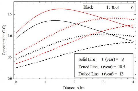
Figure 4 demonstrates the concentration distribution with in the study domain computed with parameters a=0.1 and n=0.1. Source acts up to time t(year)=8.5 and then eliminated. Dimensionless inlet boundary concentrations c/c0 are nearly 1.07, 0.57 and 0.35 at times t(year)=9, 10.5, and 12, respectively, for ξ=0 and same is recorded nearly 0.94, 0.46 and 0.25 for ξ=1. This decreasing pattern of concentration is due to no concentration introduced after the time t0=8.5. It may be noticed that rehabilitation of concentration in the semi–infinite domain is due to dispersion and advection phenomena. Unlike the uniform input concentration level reduces gradually with time at inlet boundary.
Figure 4. Solute concentration profile obtained from Eqns. (23b) and (25b) for different times in time domain t>t0
Figure 5 depicts the effect of parameter a on concentration profiles at time t(year)=9 and for n=1 on the elimination of source. Dimensionless concentration c/c0 remains higher for higher value of a throughout the study domain for steady values of all other parameters. This is because concentration, introduced to domain in presence of source up to the time 8.5, is higher for higher value of a. The concentration profile decreases with ξ but profile pattern is recorded nearly same for both ξ. It may be noticed that concentration profile is nearly parallel for fixed $\alpha$ and different ξ.
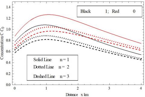
Figure 6 depicts effect of parameter n on concentration distribution after elimination of source at time t(year)=9 and for parameter a=0.1 in absence of source. As parameter n increases the concentration decreases at origin in presence of source keeping all other parameters steady, same pattern is recorded in absence of source i.e., at a particular time concentration at source end is higher for lower n. Since injected input decreases as the n increases in presence of source, the level of concentration decreases with increment n in absence source too for both ξ. For a specified time and parameter n the concentration pattern remains nearly parallel for both ξ and concentration level increases from ξ=1 to ξ=0 for a fixed n.
Figure 5. Solute concentration profile obtained from Eqns. (23b) and (25b) for different values of parameter a in time domain t>t0
Figure 6. Solute concentration profile obtained from Eqns. (23b) and (25b) for different values of parameter n in time domain t>t0
Concentration distribution has been studied mathematically (analytical solution) and later brief graphical discussion of derived result has also been attempted here. Solution is obtained for first and third type time dependent inlet boundary conditions. The developed analytical solution for semi-infinite domain clarifies how parameters influence the transport in a porous media with Cartesian coordinate. The Laplace Integral Transform Technique is used to obtain the analytical solution. Boundary conditions were set as time-dependent at the inlet and zero gradients at the outlet end. In order to obtain, solution, new independent variables introduced through separate transformations at the different stages, the variable coefficients were transformed into constant coefficients. The step-size input of varying nature where injected source produces extra amount of contaminant after certain a duration. Actually, the present work extends the result of Yadav and Roy [22] by considering scale dependent of dispersion along with non-uniform groundwater velocity and retardation factor and, varying nature input which represents real world problem more emphatically.
|
c |
concentration of solute [ML-3] |
|
ci |
resident concentration of solute [ML-3] |
|
c0 |
reference concentration of solute [ML-3] |
|
x |
distance from origin [L] |
|
X |
new space variable [L] |
|
t |
time variable [T] |
|
a |
heterogenirty parameter [L-1] |
|
R |
retardation factor at origin (dimensionless) |
|
D |
Dispersion [L2T-1] |
|
u |
groundwater velocity [LT-1] |
|
R0 |
retardation factor at origin (dimensionless) |
|
D0 |
Dispersion at origin [L2T-1] |
|
u0 |
groundwater velocity at origin [LT-1] |
|
n |
time period regulating step-size of input [T] |
|
t0 |
time up to input source acts [T] |
|
a |
parameter to regulate input increment at every step-size [ML-3] |
|
ξ |
exponents (dimensionless) that determines the relation among dispersion, velocity & retardtion |
[1] Yeh, G.T. (1981). AT123D: Analytical transient one-, two-, and three-dimensional simulation of waste transport in the aquifer system. 1439 Rep. ORNL-5602, Union Carbide Corporation for the U.S. Dept. of Energy, Oak Ridge, TN. https://doi.org/10.2172/6531241
[2] Selvadurai, A.P.S. (2004). On the advective-diffusive transport in porous media in the presence of time-dependent velocities. Geophys. Res. Lett., 31(13): L1350. https://doi.org/10.1029/2004GL019646
[3] Singh, M.K., Mahato, N.K., Singh, P. (2008). Longitudinal dispersion with time dependent source concentration in semi infinite aquifer. Journal of Earth System Science, 117: 945-949.https://doi.org/10.1007/s12040-008-0079-x
[4] Yadav, R.R., Jaiswal, D.K., Gulrana, Yadav, H.K. (2010). Analytical solution of one dimensional temporally dependent advection-dispersion equation in homogeneous porous media. International Journal of Engineering, Science and Technology, 2(5): 141-148.
[5] Jaiswal, D.K., Yadav, R.R., Gulrana. (2013). Solute-Transport under Fluctuating Groundwater Flow in Homogeneous Finite Porous Domain. J Hydrogeol Hydrol Eng., 2: 1. http://doi.org/10.4172/2325-9647.1000103
[6] Serrano, S.E. (1992). The form of the dispersion equation under recharge and variable velocity and its analytical solution. Water Resource Research, 28(7): 1801-1808. https://doi.org/10.1029/92WR00665
[7] Logan, J.D. (1996). Solute transport in porous media with scale dependent dispersion and periodic boundary conditions. J. Hydrol., 184(3-4): 261-276. https://doi.org/10.1016/0022-1694(95)02976-1
[8] Dagan, G. (1989). Flow and Transport in Porous Formations. Springer, Berlin. https://doi.org/10.1007/978-3-642-75015-1
[9] Huang, K., Van Genuchten, M.T., Zhang, R.D. (1996). Exact solutions for one-dimensional transport with asymptotic scale-dependent dispersion. Appl. Math. Model., 20(4): 298-308. https://doi.org/10.1016/0307-904X(95)00123-2
[10] Barry, D.A., Sposito, G. (1989). Analytical solution of a convection-dispersion model with time-dependent transport coefficient. Water Resour. Res., 25: 2407-2416. https://doi.org/10.1029/WR025i012p02407
[11] Basha, H.A., El-Habel F.S. (1993). Analytical solution of the one dimensional time-dependent transport equation. Water Resour. Res., 29(9): 3209-3214. https://doi.org/10.1029/93wr01038
[12] Gao, G.Y., Zhan, H.B., Feng, S.Y., Fu, B.J., Ma, Y., Huang, G.H. (2010). A new mobile-immobile model for reactive solute transport with scale-dependent dispersion. Water Resour. Res., 46(8): W08533. https://doi.org/10.1029/2009WR008707
[13] Pedretti, D., Molinari, A., Fallico, C., Guzzi, S. (2016). Implications of the change in confinement status of a heterogeneous aquifer for scale-dependent dispersion and mass-transfer processes. J. Contam. Hydrol., 193: 86-95. https://doi.org/10.1016/j.jconhyd.2016.09.005
[14] Kumar, A., Yadav, R.R. (2014). One-dimensional solute transport for uniform and varying pulse type input point source through heterogeneous medium. Environmental Technology, 36(4): 487-495. https://doi.org/10.1080/09593330.2014.952675
[15] Jaiswal, D.K., Kumar, A., Kumar, N., Yadav, R.R. (2009). Analytical solutions for temporally and spatially dependent solute dispersion of pulse type input concentration in one-dimensional semi-infinite media. Journal of Hydro-environment Research, 2(4): 254-263. https://doi.org/10.1016/j.jher.2009.01.003
[16] Bharati V.K., Sanskrityayn, A., Kumar, N. (2015). Analytical solution of ADE with linear spatial dependence of dispersion coefficient and velocity using GITT. Journal of Groundwater Research, 3: 13-26.
[17] Guerrero, J.S.P., Pimentel, L.C.G., Skaggs, T.H., van Genuchten, M.T. (2009). Analytical solution of the advection-diffusion transport equation using a change-of-variable and integral transform technique. Int. J. Heat Mass Transf., 52(13-14): 3297-3304. https://doi.org/10.1016/j.ijheatmasstransfer.2009.02.002
[18] Belyaev, A.Y., Dzhamalov, R.G., Medovar, Y.A., Yushmanov, I.O. (2007). Assessment of groundwater inflow in urban territories. Water Resour., 34(5):496-500. https://doi.org/10.1134/S0097807807050028
[19] Sharma, P.K., Abgaze, T.A. (2015). Solute transport through porous media using asymptotic dispersivity. Indian Academy of Sciences, 40(5): 1595-1609. https://doi.org/10.1007/s12046-015-0382-6
[20] You, K.H., Zhan, H.B. (2013). New solutions for solute transport in a finite column with distance-dependent dispersivities and time-dependent solute sources. J. Hydrol., 487: 87-97. https://doi.org/10.1016/j.jhydrol.2013.02.027
[21] Sanskrityayn, A., Suk, H., Kumar, N. (2017). Analytical solutions for solute transport in groundwater and riverine flow using Green’s Function Method and pertinent coordinate transformation method. Journal of Hydrology, 547: 517-533. https://doi.org/10.1016/j.jhydrol.2017.02.014
[22] Yadav, R.R., Roy, J. (2018). Solute transport phenomena in a heterogeneous semi-infinite porous media: An analytical solution. Int. J. Appl. Comput. Math, 4: 135. https://doi.org/10.1007/s40819-018-0567-x
[23] Yadav, R.R., Yadav, V. (2019). Three-dimensional analytical models for time-dependent coefficients through uniform and varying plane input source in semi-infinite adsorbing porous media. Pollution, 5(1): 81-98. https://doi.org/10.22059/poll.2018.258411.445
[24] Bear, J. (1972). Dynamics of Fluid in Porous Media. Elsevier Publication Co., New York.
[25] Freeze, R.A., Cherry, J.A. (1979). Groundwater. Prentice-Hall, Englewood Cliffs, N.J.
[26] Yim, C.S., Mohsen M.F.N. (1992). Simulation of tidal effects on contaminant transport in porous media. Ground Water, 30(1): 78-86. https://doi.org/10.1111/j.1745-6584.1992.tb00814.x
[27] Scheidegger, A.E. (1957.). The Physics of Flow Through Porous Media. Toronto, Canada: University of Toronto Press.
[28] Pickens, J.F., Grisak, G.E. (1981). Modeling of scale dependent dispersion in hydrogeologic systems. Water Resour. Res., 17(6): 1701-1711. https://doi.org/10.1029/WR017i006p01701
[29] Chatterjee, A. Singh, M.K. (2017). Two-dimensional advection-dispersion equation with depth-dependent variable source concentration. Pollution, 4(1): 1-8. https://doi.org/10.22059/poll.2017.230145.265
[30] Yadav, R.R., Kumar, L.K. (2017). One-dimensional spatially dependent solute transport in semi-infinite porous media: An analytical solution. International Journal of Engineering, Science and Technology, 9(4):20-27. https://doi.org/10.4314/ijest.v9i4.3
[31] Yadav, R.R., Jaiswal, D.K., Gulrana, Yadav, H.K. (2010). Analytical solution of one dimensional temporally dependent advection-dispersion equation in homogeneous porous media. International Journal of Engineering, Science and Technology, 2(5): 141-148. https://doi.org/10.4314/ijest.v2i5.60133
[32] Todd, D.K. (1980). Groundwater Hydrology. John Wiley, New York, USA.