Maher A. Jasim*![]() | Ali Ben Ahmed
| Ali Ben Ahmed![]()
© 2025 The authors. This article is published by IIETA and is licensed under the CC BY 4.0 license (http://creativecommons.org/licenses/by/4.0/).
OPEN ACCESS
Understanding how electrons are arranged in titanium, aluminum, and compounds made from both is very important for improving materials used in airplanes, designing stronger materials, and making better catalysts. This is because electron arrangement affects how strong a material is, how well it resists rust, and how it reacts with other chemicals. But, it's hard to figure out the exact electron arrangement in these materials because electrons interact with each other in complicated ways, and our current theories aren't perfect. This work tries to: (1) find the most likely electron arrangements for titanium and aluminum using computer simulations, (2) check if a specific model (the Renormalized Free Atom or RFA model) matches experimental data, and (3) estimate the electron arrangement in a TiAl₃ alloy by combining the results for titanium and aluminum. We computed how electrons move in titanium and aluminum using the RFA model, testing different electron arrangements for titanium's 3d-4s and aluminum's 3s-3p electrons. We then computed Compton scattering profiles J(pz) and compared them with experiment to see how well the model works. For the TiAl₃ alloy, the electron arrangement is estimated by adding the arrangements we found for both pure titanium and aluminum. Results demonstrated well matched calculations for both RFA and the experimental data. Electron arrangements are mostly found to be 3d³-4s¹ and 3s²-3p¹ for titanium and aluminum, respectively. Predicting how electrons move in the TiAl₃ alloy was achieved by superposition model, that matches experimental data. This shows the efficiency of applying RFA model to predict the electronic properties of titanium-aluminum systems and helps to design new and better titanium-aluminum compounds.
aluminum, titanium, TiAl3 alloy, Compton profile (CP), superposition model, Compton scattering
Compton scattering is can be explained as an inelastic photon-electron interaction, causing the exchange of energy and momentum. Subsequently, the scattered photon’s properties depend on the electron’s initial state with which it interacts. Then, the photon momentum distribution becomes the exact mirror image of the electron momentum distribution before collision [1]. The so-called Compton profile presents the function describing the electron momentum distribution in this scenario. Investigating the electronic structure of a great majority of solids, crystallized material in particular can be effectively realized by Compton spectroscopy Valuable information regarding the electron momentum density (EMD) can be gained, which is very useful in measuring electron wave functions by means of Fourier transform equations [2]. The electrons in solids are classified into two groups: inner core and conduction electrons. The first type is bound and localized close to the atomic nucleus. They take little or no part in bonding. The conduction electrons, on the contrary, are rather more loosely bound with their radial wave functions extended sufficiently far to form a significant contribution toward bonding and electrical conduction [3]. Following the initial discovery of the Compton effect, early quantitative experiments sought to measure the energy distribution of scattered photons, focusing on the Compton cross section. Researchers like Dumond and Kirkpatrick meticulously analyzed such data, establishing how the width of the Compton spectral line correlates with the electron momentum distribution. Overall, Compton scattering remains a valuable method for investigating electron distributions across atoms, molecules, and condensed matter surfaces [4]. In 2018, Sankarshan and Umesh [5] he pointed out that during the scattering of X-rays and gamma rays from amorphous media, especially at high momentum transfer, each atom in which it occurs is scattered individually without noticing the presence of other atoms in its vicinity. In Weiss's scattering experiment, this is equivalent to a practical situation where the operator can set up the angular assembly of the photon source and scatterer so that the incoming energy exceeds the electron binding energy of the scatterer atoms, and a scattering angle large enough to achieve high momentum transfer is used. We can interpret Weiss's conclusion that under these conditions the following occurs: (a) all targets behave as pure incoherent distractors and (b) complex targets can be treated as either homogeneous or heterogeneous mixtures of elements [5].
In the early nineteenth century, the Compton effect was discovered, which provides a fundamental explanation for the laws of conservation of energy and momentum in quantum mechanical processes [6].
Compton scattering is an experimental capability that can be employed to explore the electron momentum distribution in matter, and through CS, the chemical character can be correlated with the electronic structure via the electron momentum density n(p). Compton profile (CP) J(pz) is one-dimensional quantity—and is the projection of the three-dimensional momentum density n(p) onto the scattering vector (parallel to pz). Mathematical approach states that the momentum density n(p) is "smoothed" along the directions orthogonal to pz, and n(pz) = n(p,φ) with polar coordination [7-25].
The Compton profile is a one-dimensional view of how electrons move in three dimensions along the scattering vector can be realized by Compton profile shows. This can be explained as integrating electron movement over components not parallel to the vector. This reduces the momentum distribution to one dimension. The electron distribution in a material's momentum space can be shown in the profile, with characteristic features relate to valence and core electrons. The scattered photon energies relate to momentum distribution can be realized by measuring scattered high-energy photons, hence the electronic structure is obtaied. The math relationship between the Compton profile J(Pz) and electron momentum density n(p) is viewed as:
$J\left(P_Z\right)=\iint n(p) d p_x d p_y$
where, pz represents the momentum component aligned with the scattering vector, the integral accounts for perpendicular components px and py. This integral equation is key to interpreting Compton scattering experiments and supports the theoretical calculations in this work.
Materials science still struggles to pinpoint the electronic structure of titanium, aluminum, and their intermetallic compounds such as TiAl₃. Earlier Compton scattering work gave helpful experimental insight, but theoretical models usually use free-atom approximations. These don't fully explain electron behavior and renormalization, especially in alloys and intermetallic systems. Because of these limits, there are often differences between the calculated and experimental electron momentum densities. This hurts the ability of current theoretical frameworks to make predictions. Though much research has been done on pure elemental metals, there aren't as many investigations as possible into the electronic structure of titanium-aluminum alloys using strong theoretical methods. By adding renormalization effects into the atomic wavefunctions, the Renormalized Free Atom (RFA) model gives a better theoretical method that more closely matches experimental results. But, using it on titanium, aluminum, and TiAl₃ alloys hasn't been explored much. This work aims to fix this by using the RFA model to get the best electronic layouts of Ti and Al, checking these layouts against experimental Compton profiles, and using this method to guess the electronic structure of TiAl₃ via a superposition model. This research not only makes the electronic configuration assignments for the elements better, but it also creates a checked computational framework for alloy electronic structure. It improves the theoretical way we understand titanium-aluminum intermetallic.
This study seeks to: (1) compute titanium and aluminum's electronic momentum density and Compton profiles using the Renormalized Free Atom (RFA) model; (2) spot the best electronic setups for Ti and Al by matching theory with Compton scattering experiments; and (3) use these results to model the electronic structure of the TiAl₃ intermetallic alloy using a superposition model based on the best elemental setups. Consequently, this study aims at fixing problems with older theoretical methods that often can't correctly guess electron momentum densities in elements and alloys. The othe goal is to offer a tested computational method that enhances knowledge of electronic structure of Ti-Al systems.
2.1 Calculations (RFA) model
Berggren’s approach is used to compute CP of polycrystalline (Ti, Al) using RFA model. Since the scheme of computing RFA CP of valence electrons is available in the study [26], we give a few computational details.
Berggren's method gives a way to figure out the momentum-space wavefunctions for valence electrons in crystals, hence finding the electron momentum density in the Renormalized Free Atom (RFA) model. The electron Bloch wavefunctions change into momentum space, especially for the outermost s-electrons, by presenting them as combinations of plane waves. These waves have momenta around reciprocal lattice vectors. This change helps compute Compton profiles by allowing integration over momentum parts. The RFA model uses Berggren’s method to get wavefunctions in momentum-space that include renormalization stuff. This is because atomic wavefunctions cut off at the Wigner-Seitz sphere boundary. Putting Berggren’s momentum transform into the RFA model improves how we theoretically predict electron momentum densities and compare them with Compton scattering data from experiments.
HF wave function for 4s electron of (Ti, Al) obtained from literature [27]. It has been truncated at WS radius and then renormalized to unity. The new wave function is then used in further computations. It has been known [28] that the effects of renormalization are the largest for the outermost 's' electrons because hardly 25-35% charge is contained in W-S sphere. On the other hand, for '3d' electrons this figure is about 90% and thus renormalization effects on 3d electrons are very small. Following the above, we have also considered 4s electrons only in the RFA scheme. The Compton profile J4S(pz) due to only 4s electrons was computed as
$\mathrm{J}_{4 s}\left(p_z\right)=4 \pi \sum_{n=0}^{\infty}\left|\Psi_0^c\left(K_n\right)\right|^2 G_n\left(p_z\right)$ (1)
where, $\Psi_0^c\left(K_n\right)$ is the FT of the RFA and $G_n\left(P_z\right)$ is an auxiliary function involving reciprocal lattice vectors $K_n$, number of points in the $n^{\text {th}}$ shell, Fermi momentum $p_F$, etc.
2.2 Calculations (superposition) model
The superposition model is a simple and successful model used to find the shape of the Compton curve (Jpz) for alloys. It depends on the results of theoretical calculations of the alloying elements. The data for the elements are collected in different proportions using the following equation [29]:
$J^{S U P \cdot}\left(p_z\right)=C J^{T i}\left(p_z\right)+D J^{A l}\left(p_z\right)$ (2)
where, C and D represent the concentration ratios of the elements titanium (Ti) and aluminum (Al) respectively in the alloy.
3.1 Titanium
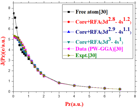
Table 1 contains the results of theoretical calculations for the Compton profile (Jpz) of titanium, in addition to the experimental values results for (Jpz) [30], as these values represent the electronic structures closest to the approved experimental values results. The values of the Compton profile (Jpz) closest to the experimental data of titanium are the electronic compositions: (3d3 4s1), (3d2.9 4s1.1), (3d2.8 4s1.2) which has been calibrated to the area under the curve of the free atom (9.921118) for the momentum region bounded between (0- 0.7 a.u.).
Table 1. Comparison of theoretical and experimental results of the Compton profile for (Ti)
|
Pz (a.u.) |
J(pz)(e/a.u.) |
|||||
|
Free atom (3d2- 4s2) [27] |
Theor.Core+(RFA) |
Data (PW-GGA) [30] |
Expt. [30] |
|||
|
Core+RFA 3d2.8- 4s1.2 |
Core+RFA 3d2.9- 4s1.1 |
Core+RFA 3d3- 4s1 |
||||
|
0.0 |
7.51 |
5.235 |
5.263 |
5.294 |
5.236 |
5.359±0.014 |
|
0.1 |
7.1 |
5.214 |
5.241 |
5.27 |
5.221 |
5.331 |
|
0.2 |
6.14 |
5.12 |
5.141 |
5.163 |
5.172 |
5.249 |
|
0.3 |
5.16 |
4.955 |
4.964 |
4.974 |
5.088 |
5.119 |
|
0.4 |
4.46 |
4.772 |
4.771 |
4.769 |
4.947 |
4.941 |
|
0.5 |
4.04 |
4.538 |
4.526 |
4.508 |
4.753 |
4.717 |
|
0.6 |
3.8 |
4.168 |
4.132 |
4.088 |
4.522 |
4.456 |
|
0.7 |
3.64 |
3.863 |
3.869 |
3.875 |
4.262 |
4.173 |
|
0.8 |
3.48 |
3.706 |
3.712 |
3.718 |
3.996 |
3.882 |
|
1.0 |
3.15 |
3.341 |
3.346 |
3.352 |
3.458 |
3.320±0.010 |
|
1.2 |
2.77 |
2.936 |
2.94 |
2.945 |
2.906 |
2.835 |
|
1.4 |
2.39 |
2.533 |
2.536 |
2.539 |
2.412 |
2.408 |
|
1.6 |
2.04 |
2.165 |
2.167 |
2.169 |
2.033 |
2.064 |
|
1.8 |
1.74 |
1.844 |
1.845 |
1.846 |
1.739 |
1.793 |
|
2 |
1.5 |
1.576 |
1.576 |
1.577 |
1.504 |
1.547±0.006 |
|
3 |
0.839 |
0.869 |
0.868 |
0.867 |
0.823 |
0.857±0.005 |
|
4 |
0.596 |
0.606 |
0.605 |
0.604 |
0.590 |
0.584±0.004 |
|
5 |
0.447 |
0.453 |
0.451 |
0.44 |
0.444 |
0.438±0.003 |
|
6 |
0.335 |
0.338 |
0.337 |
0.335 |
0.333 |
0.328±0.002 |
|
7 |
0.251 |
0.254 |
0.253 |
0.250 |
0.250 |
0.254±0.002 |
The theoretical calculations were compared with the experimental values results to find out the extent of their congruence, as we note that the values obtained using the (RFA) model match well with the experimental values results, and that the best match is found in the electronic arrangement (3d3- 4s1).
As can be seen in momentum region (0-1 a.u.), the experimental values results are slightly higher than the theoretical results, but in the momentum region confined between (1.2-6 a.u.) we notice that the theoretical results become slightly higher than the experimental values results, and this applies to theoretical calculations for RFA models.
As for the values of the free atom, they are much lower and far from the experimental values adopted [27] in the momentum region (0-1 a.u.), but they come back close to them in the momentum region (1.2-7 a.u.).
Figure 1 represents a comparison between theory and experiments given in Table 1, as we note that the theoretical results match well with the experimental values results [30].
Figure 1. Comparison between theoretical and experimental CP for Ti
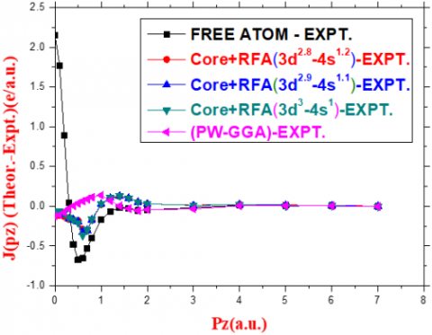
As we note that the least difference between the results of theoretical calculations and experimental values results is (0.3940886, 0.384615, 0.3726636), which corresponds to the electronic arrangement (3d3-4s1, 3d2.9 4s1.1, 3d2.8 4s1.2), which represents the optimal electronic arrangement and the closest to experimental values results [30].
Figure 2 includes drawing the differences between the results of the theoretical calculations and the results of the experimental values results. In order to determine the optimal electronic composition and the closest to the experimental values results, the differences between the theoretical and practical values have been calculated using the following relationship:
$\left(\sum_0^7\left(J_{\text {Theo.}}\left(p_z\right)-J_{\text {exp.}}\left(p_z\right)\right)\right)^2=\sum_0^7\left|\Delta J\left(p_z\right)\right|^2$ (3)
Figure 2. Difference between theoretical and experimental results [30]
The electronic arrangement (3d3-4s1) of the (RFA) model takes the least differences, which is equal to (0.3940886), because it is the electronic arrangement closest to the approved experimental values results [30].
CP of polycrystalline of (Ti). All theoretical Normalized of (9.921118) electrons.
3.2 Aluminum
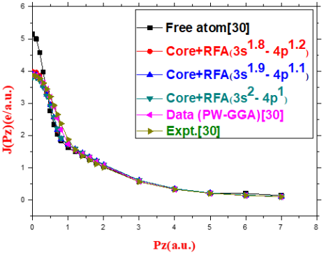
Table 2 shows the values of the theoretical results of the (RFA) model and of the electronic arrangements closest to the experimental values.
Table 2 contains the electronic arrangements close to the approved experimental values results [30], which were obtained from the calculations of the RFA model, as all values were calibrated to the area under the curve for the free atom is (5.78352) within the limits of the Wigner-Seitz sphere and for the momentum region confined between (0→7 a.u.).
Table 2. Comparison of theoretical and experimental results of the Compton profile for (Al)
|
Pz (a.u.) |
J(pz) (e/a.u.) |
|||||
|
Free atom (3s2- 3p1) [27] |
Theory(RFA) |
Data (PW-GGA) [30] |
Expt. [30] |
|||
|
Core+RFA 3s1.8- 4p1.2 |
Core+RFA 3s1.9- 4s1.1 |
Core+RFA 3s2- 3p1 |
||||
|
0.0 |
5.15 |
3.974 |
3.897 |
3.816 |
3.880 |
3.871 ± 0.021 |
|
0.1 |
5 |
3.958 |
3.882 |
3.803 |
3.853 |
3.844 |
|
0.2 |
4.57 |
3.852 |
3.781 |
3.708 |
3.769 |
3.766 |
|
0.3 |
3.97 |
3.611 |
3.552 |
3.493 |
3.628 |
3.631 |
|
0.4 |
3.32 |
3.307 |
3.267 |
3.226 |
3.435 |
3.441 |
|
0.5 |
2.76 |
2.969 |
2.95 |
2.929 |
3.191 |
3.204 |
|
0.6 |
2.34 |
2.56 |
2.563 |
2.563 |
2.889 |
2.936 |
|
0.7 |
2.04 |
2.158 |
2.182 |
2.203 |
2.539 |
2.652 |
|
0.8 |
1.84 |
1.884 |
1.888 |
1.911 |
2.183 |
2.368 |
|
1.0 |
1.62 |
1.703 |
1.714 |
1.725 |
1.734 |
1.876 ± 0.013 |
|
1.2 |
1.49 |
1.562 |
1.575 |
1.587 |
1.531 |
1.554 |
|
1.4 |
1.38 |
1.438 |
1.451 |
1.464 |
1.419 |
1.361 |
|
1.6 |
1.26 |
1.318 |
1.329 |
1.34 |
1.303 |
1.236 |
|
1.8 |
1.14 |
1.196 |
1.207 |
1.217 |
1.182 |
1.113 |
|
2 |
1.03 |
1.077 |
1.086 |
1.096 |
1.063 |
1.011 ± 0.009 |
|
3 |
0.568 |
0.601 |
0.606 |
0.611 |
0.570 |
0.557 ± 0.007 |
|
4 |
0.322 |
0.341 |
0.344 |
0.347 |
0.323 |
0.324 ± 0.005 |
|
5 |
0.199 |
0.211 |
0.213 |
0.215 |
0.199 |
0.198 ± 0.003 |
|
6 |
0.199 |
0.141 |
0.143 |
0.144 |
0.133 |
0.134 ± 0.003 |
|
7 |
0.134 |
0.098 |
0.1 |
0.102 |
0.094 |
0.095 ±0.002 |
The results of the theoretical calculations were compared with the values of the experimental values to find out the extent of their compatibility, as we note that the values obtained using the (RFA) model correspond well with the practical values, and that the best match is found in the electronic arrangement (3s2 - 3p1).
It can also be seen that in the region (0→1 a.u.) the practical data are slightly higher than the theoretical results, but in the momentum region confined between (1.2→7 a.u.) we notice that the theoretical results become slightly higher than the practical values [6]. This applies to the theoretical calculations of both (RFA) and (FE) model.
Figure 3 shows the wave function of the free atom with the wave functions of the theoretical values of the (RFA) model in addition to the wave function of the experimental values, as it can be noted that the wave functions of the calculated theoretical values are in line with the wave function For experimental values more than the wave function of the free atom and Figure 3 shows the comparison between the results of theoretical calculations and the experimental values [30] for the Compton profile of aluminum, as we note that the values of the (RFA) model correspond well with the experimental values, especially the electronic arrangement (3s2 - 3p1). of the (RFA) model, as the arrangement is the best and most compatible.
Figure 3. Comparison between calculated and experimental CP for Al
Regarding the measurements for the free atom, these differ substantially from the observed experimental data within the low momentum range (0 to 0.3 a.u.), where the free atom’s values are notably greater. However, as momentum approaches 0.4 a.u., the theoretical and experimental results start to align again. Beyond this point, specifically in the interval between 0.5 and 1.2 a.u., the free atom values actually fall below those recorded in experiments.
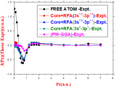
As we note that the least difference between the results of theoretical calculations and experimental values results is (0.6636685, 0.6743779, 0.7460561), which corresponds to the electronic arrangement (3s2 - 3p1, 3s1.9 - 3p1.1, 3s1.8 - 3p1.2), which represents the optimal electronic arrangement and the closest to experimental values [30].
Figure 4 represents the values of the differences between the results of the theoretical calculations and the experimental data of the Compton profile (Jpz), as the electronic arrangement (3s2- 3p1) of the (RFA) model takes the least differences, which is equal to (0.6636685), because it is the electronic arrangement closest to the experimental values approved [30].
Figure 4. Graph showing the disparity between calculated and measured Compton profiles for polycrystalline Al
3.3 TiAl3 alloy
The theoretical results for the shape of the Compton Profile (JPz) of the alloy (TiAl3) were found using the superposition model using equation (2). The calculations were made based on the theoretical results for the shape of the CP of (Ti) and (Al) completely, considering the proportion of each element.
Table 3. Theoretical calculations and practical measurements for the shape of the Compton curve (JPz) for the elements titanium (Ti) and aluminum (Al) as well as the alloy (TiAl3) and for the momentum region between (0→7 a.u.)
|
Pz (a.u.) |
J(pz) (e/a.u.) |
||||||
|
Ti |
Al |
Superposition Model TiAl3 |
|||||
|
RFA 3d3- 4s1 |
RFA 3s2- 3p1 |
Free atom [27] |
Present Work. RFA |
Alloy (PW-GGA) [30] |
Sup (PW-GGA) [30] |
Expt. [30] |
|
|
0.0 |
5.294 |
3.816 |
22.96 |
16.695 |
17.395 |
16.877 |
16.618±0.038 |
|
0.1 |
5.27 |
3.803 |
22.1 |
16.63 |
17.266 |
16.780 |
16.466 |
|
0.2 |
5.163 |
3.708 |
19.85 |
16.239 |
16.884 |
16.482 |
16.148 |
|
0.3 |
4.974 |
3.493 |
17.07 |
15.407 |
16.297 |
15.973 |
15.667 |
|
0.4 |
4.769 |
3.226 |
14.42 |
14.405 |
15.577 |
15.255 |
14.96 |
|
0.5 |
4.508 |
2.929 |
12.32 |
13.255 |
14.714 |
14.327 |
14.047 |
|
0.6 |
4.088 |
2.563 |
10.82 |
11.741 |
13.593 |
13.192 |
13.038 |
|
0.7 |
3.875 |
2.203 |
9.76 |
10.448 |
12.203 |
11.880 |
12.01 |
|
0.8 |
3.718 |
1.911 |
9 |
9.417 |
10.664 |
10.545 |
10.96 |
|
1.0 |
3.352 |
1.725 |
8.01 |
8.496 |
8.345 |
8.662 |
8.980±0.028 |
|
1.2 |
2.945 |
1.587 |
7.24 |
7.68 |
7.215 |
7.501 |
7.613 |
|
1.4 |
2.539 |
1.464 |
6.53 |
6.908 |
6.487 |
6.670 |
6.534 |
|
1.6 |
2.169 |
1.34 |
5.82 |
6.172 |
5.812 |
5.942 |
5.811 |
|
1.8 |
1.846 |
1.217 |
5.16 |
5.481 |
5.157 |
5.286 |
5.167 |
|
2 |
1.577 |
1.096 |
4.59 |
4.851 |
4.562 |
4.695 |
4.611±0.019 |
|
3 |
0.867 |
0.611 |
2.543 |
2.693 |
2.520 |
2.534 |
2.594±0.014 |
|
4 |
0.604 |
0.347 |
1.562 |
1.64 |
1.559 |
1.561 |
1.582±0.010 |
|
5 |
0.44 |
0.215 |
1.044 |
1.09 |
1.041 |
1.044 |
1.053±0.008 |
|
6 |
0.335 |
0.144 |
0.737 |
0.764 |
0.732 |
0.735 |
0.768±0.007 |
|
7 |
0.250 |
0.102 |
0.535 |
0.554 |
0.531 |
0.534 |
0.559±0.005 |
Table 3 shows the calculated results of the shape of the CP (JPz) for the alloy (TiAl3) according to the free atom recalibration (RFA) and free atom (FA) models, which were found using the superposition model. These theoretical results were compared with the results of the practical measurements [30] for this alloy.
Table 3 represents the values of the theoretical and practical calculations for the shape of the Compton Profile (JPz) for the alloy (TiAl3). Theoretical values of (JPz) for the alloy were calculated using theoretical values of (JPz) for the elements (Ti) and (Al). Also, the two electronic arrangements (3d3 4s1) and (3s2 3p1) were chosen for the elements (Ti) and (Al), respectively to form the alloy (TiAl3), since these two arrangements represent the best choice and the closest to the outcome of practical measurements. Theoretical Compton Profile for the alloy (TiAl3) was found to be comparable with the those of actual measurements [30] for this alloy.
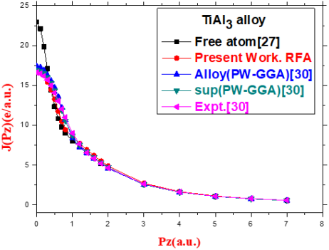
Figure 5 displayed the shape of the Compton Profile for both the theoretical calculations and the practical measurements for the alloy (TiAl3). The ratio of the alloy (TiAl3) shows that the ratio of Al is three times that of Ti. All theoretical calculations and practical measurements [30] of the shape of the Compton Profile (JPz) were performed using (a.u.) unit for the momentum region between (0→7 a.u.).
Figure 5. The experimental values of J(pz) against pz (a.u.) for (TiAl3)
The electronic configurations (3d3 4s1) and (3s2 3p1) of the elements titanium (Ti) and aluminum (Al) respectively, which are closest to the approved practical values [30], were found using the free atom recalibration (RFA) model, i.e. the optimal electronic configurations closest to the practical measurements are similar for both the (RFA) and (FA) models.
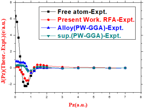
Figure 6. Comparison between the theoretical and experimental values of J(pz) for (TiAl3)
Figure 6 includes a graph showing the amount of differences between the results of theoretical calculations and the results of practical measurements of (JPz) for the alloy (TiAl3), as Eq. (4) was used to find the values of these differences.
Titanium: The EMD of the Ti was studied using the (RFA) model, and the results were in comparable with the values of the approved experimental measurements. The RFA model can satisfactory reproduce the experiment results in the (3d3- 4s1) configuration.
Aluminum: The EMD of Al was studied using the (RFA) approach, and the outcomes closely matched the findings from validated experimental data. The RFA technique demonstrated strong consistency with observational results, particularly for the (3s²-3p¹) electronic configuration.
TiAl3 alloy: The shape of the Compton profile (Jpz) of the alloys was calculated using the S.P.Model, which is based on the theoretical results of the Compton curve (Jpz) of the elements titanium (Ti) and aluminum (Al). The best electronic arrangements obtained using the RFA models for the two elements were selected and entered as computational data in the S.P.Model to form the alloy. The findings obtained from the S.P. Model were evaluated against the experimental data for the TiAl3 alloy, revealing that the theoretical predictions closely matched the measured results for this material.
[1] Agui, A., Harako, A., Shibayama, A., Haishi, K., et al. (2019). Temperature dependence of the microscopic magnetization process of Tb12Co88 using magnetic Compton scattering. Journal of Magnetism and Magnetic Materials, 484: 207-211. https://doi.org/10.1016/j.jmmm.2019.04.031
[2] Aguiar, J.C., Mitnik, D., DiRocco, H.O. (2015). Electron momentum density and Compton profile by a semi-empirical approach. Journal of Physics and Chemistry of Solids, 83: 64-69. https://doi.org/10.1016/j.jpcs.2015.03.023
[3] Ekman, M., Ozoliņš, V. (1998). Electronic structure and bonding properties of titanium silicides. Physical Review B, 57(8): 4419. https://doi.org/10.1103/PhysRevB.57.4419
[4] Wan, J.J., Gu, J., Wu, Z.Y., Wu, F., Li, J., Qiao, H.X. (2023). High-accuracy calculation of nonrelativistic Compton profile for H-like ions. Results in Physics, 50: 106562. https://doi.org/10.1016/j.rinp.2023.106562
[5] Sankarshan, B.M., Umesh, T.K. (2018). Compton profiles of some composite materials normalized by a new method. Radiation Physics and Chemistry, 144: 106-110. https://doi.org/10.1016/j.radphyschem.2017.12.001
[6] Sekania, M., Appelt, W.H., Benea, D., Ebert, H., Vollhardt, D., Chioncel, L. (2018). Scaling behavior of the Compton profile of alkali metals. Physica A: Statistical Mechanics and its Applications, 489: 18-27. https://doi.org/10.1016/j.physa.2017.07.018
[7] Park, S.D., Kim, S.Y. (2023). First-principles study on the electronic and mechanical properties of the Cr (001)/Al (001) structure. ACS Omega, 8(45): 42840-42848. https://doi.org/10.1021/acsomega.3c05827
[8] Yang, Y., Hiraoka, N., Matsuda, K., Holzmann, M., and Ceperley, D.M. (2020). Quantum Monte Carlo Compton profiles of solid and liquid lithium. Physical Review B, 101(16): 165125. https://doi.org/10.1103/PhysRevB.101.165125
[9] Şakar, E., Akbaba, U., Zukowski, E., and Gürol, A. (2018). Gamma and neutron radiation effect on Compton profile of the multi-walled carbon nanotubes. Nuclear Instruments and Methods in Physics Research, Section B: Beam Interactions with Materials and Atoms, 437: 20-26. https://doi.org/10.1016/j.nimb.2018.10.027
[10] Aguiar, J.C., Quevedo, C.R., Gomez, J.M., DiRocco, H.O. (2017). Theoretical Compton profile of diamond, boron nitride and carbon nitride. Physica B: Condensed Matter, 521: 361-364. https://doi.org/10.1016/j.physb.2017.07.016
[11] Mattheiss, L.F. (1992). Calculated structural properties of CrSi2, MoSi2, and WSi2. Physical Review B: Condensed Matter and Materials Physics, 45(7): 3252-3259. https://doi.org/10.1103/physrevb.45.3252
[12] Vajeeston, P., Ravindran, P., Ravi, C., Asokamani, R. (2001) Electronic structure, bonding, and ground-state properties of AlB2-type transition-metal diborides. Physical Review B, 63: 045115. https://doi.org/10.1103/PhysRevB.63.045115
[13] Hong, T., Watson-Yang, T.J., Freeman, A.J., Oguchi, T., Xu, J. (1990). Crystal structure, phase stability, and electronic structure of Ti-Al intermetallics: TiAl3. Physical Review B, 41(18): 12462. https://doi.org/10.1103/PhysRevB.41.12462
[14] Dhaked, K., Shukla, R., Sharma, K.S., Sharma, R. (2025). Ab-initio investigation of optical and electronic-structure properties of monoclinic tungsten trioxide (WO3): A DFT approach. In Proceedings of the 1st International Conference on Materials and Thermophysical Properties, Jaipur, India, pp. 241-254. https://doi.org/10.1007/978-981-96-6795-6_28
[15] Joshi, R., Sahariya, J., Mund, H.S., Bhamu, K.C., Tiwari, S., Ahuja, B.L. (2012). Compton profiles of MoP and WP: Validation of second order generalized gradient approximation. Computational Materials Science, 53(1): 89-93. https://doi.org/10.1016/j.commatsci.2011.09.022
[16] Doublet, M.L., Remy, S., Lemoigno, F. (2000). Density functional theory analysis of the local chemical bonds in the periodic tantalum dichalcogenides TaX2 (X=S, Se, Te). The Journal of Chemical Physics, 113: 5879-5890. https://doi.org/10.1063/1.1290023
[17] Alhamedi, M.Z., Mohammed, F.M. (2022). Theoretical compton profile of fcc zinc (Zn). Materials Today: Proceedings, 61: 914-920. https://doi.org/10.1016/j.matpr.2021.09.553
[18] Meena, B.S., Heda, N.L., Kumar, K., Bhatt, S., Mund, H.S., Ahuja, B.L. (2016). Compton profiles and Mulliken’s populations of cobalt, nickel and copper tungstates: Experiment and theory. Physica B: Condensed Matter, 484: 1-6. https://doi.org/10.1016/j.physb.2015.12.035
[19] Ali, H.A., Turki, I.I., Al-Obaidy, G.S., Rzaij, J.M. (2025). Evaluating the gamma-ray attenuation characteristics of various radioactive sources using binary and ternary polymer blends. Revue des Composites et des Matériaux Avancés-Journal of Composite and Advanced Materials, 35(5): 935-945. https://doi.org/10.18280/rcma.350513
[20] Mohammed, S.F., Mohammad, F.M., Sahariya, J., Mund, H.S., Bhamu, K.C., Ahuja, B.L. (2013). Electronic structure of CaCO3: A Compton scattering study. Applied Radiation and Isotopes, 72: 64-67. https://doi.org/10.1016/j.apradiso.2012.10.006
[21] Raykar, V., Bhamu, K.C., Ahuja, B.L. (2013). Compton profile study and electronic properties of tantalum diboride. Applied Radiation and Isotopes, 77: 38-43. https://doi.org/10.1016/j.apradiso.2013.02.020
[22] Milić P., Marinković D., Klinge S., Ćojbašić Ž., 2023, Reissner-Mindlin Based Isogeometric Finite Element Formulation for Piezoelectric Active Laminated Shells, Tehnicki Vjesnik, 30(2): 416-425
[23] Dhaka, M.S., Sharma, G., Mishra, M.C., Joshi, K.B., Kothari, R.K., Sharma, B.K. (2011). Electron momentum density distribution in Cd3P2. Computer Physics Communications, 182(9): 2017-2020. https://doi.org/10.1016/j.cpc.2010.12.024
[24] Sharma, Y., Srivastava, P., Dashora, A., Vadkhiya, L., et al. (2012). Electronic structure, optical properties and Compton profiles of Bi2S3 and Bi2Se3. Solid State Sciences, 14(2): 241-249. https://doi.org/10.1016/j.solidstatesciences.2011.11.025
[25] Ko, D.S., Lee, W.J., Sul, S., Jung, C., et al. (2018). Understanding the structural, electrical, and optical properties of monolayer h-phase RuO2 nanosheets: A combined experimental and computational study. NPG Asia Materials, 10(4): 266-276. https://doi.org/10.1038/s41427-018-0020-y
[26] Courvoisier, T.J.L. (2013). Compton processes. In Courvoisier, T.J.-L. (Ed.), High Energy Astrophysics, Springer, New York, pp. 75-89. https://doi.org/10.1007/978-3-642-30970-0_6
[27] Clementi, E., Roetti, C. (1974). Roothaan-Hartree-Fock atomic wavefunctions: Basis functions and their coefficients for ground and certain excited states of neutral and ionized atoms, Z≤54. Atomic Data and Nuclear Data Tables, 14(3-4): 177-478. https://doi.org/10.1016/S0092-640X(74)80016-1
[28] Biggs, F., Mendelsohn, L.B., Mann, J.B. (1975). Hartree-Fock Compton profiles for the elements. Atomic Data and Nuclear Data Tables, 16(3): 201-309. https://doi.org/10.1016/0092-640X(75)90030-3
[29] Zou, J., Fu, C.L., Yoo, M.H. (1995). Phase stability of intermetallics in the AlTi system: A first-principles total-energy investigation. Intermetallics, 3(4): 265-269. https://doi.org/10.1016/0966-9795(95)97286-A
[30] Sharma, G., Joshi, K.B., Dhaka, M.S., Mishra, M.C., Kothari, R.K., Sharma, B.K. (2011). Compton profile and charge transfer study in intermetallic Ti–Al system. Intermetallics, 19(8): 1107-1114. https://doi.org/10.1016/j.intermet.2011.03.004