Baolei Nie | Jia Zhang![]() | Qingyan Zhang*
| Qingyan Zhang*![]()
© 2024 The authors. This article is published by IIETA and is licensed under the CC BY 4.0 license (http://creativecommons.org/licenses/by/4.0/).
OPEN ACCESS
In this paper, the stress wave propagation and attenuation laws in heterogeneous materials such as rock and concrete are investigated by equating these materials to periodic materials through the viscoelastic analogy method. Firstly, the relaxation functions and stress response curves of the periodic materials are obtained by using a novel numerical inverse transformation method based on the viscoelastic analogy theory. Then, an experimental study of stress wave propagation in slender concrete rods was carried out on a Hopkinson pressure rod platform. The results show that there is a significant attenuation trend of the stress wave during 10 times of reflections. Comparison of the numerical inverse transform results with the experimental results shows that the decay rate in the experiment is faster than that predicted by simple viscosity. Finally, the effects of geometric dispersion and frictional dissipation of energy are considered in ABAQUS finite element simulations. The finite element analysis results show that inherent viscosity in heterogeneous materials can partially explain the stress wave attenuation in concrete. The viscoelastic simulation method effectively predicts stress wave attenuation in heterogeneous materials and provides theoretical insights for engineering applications.
stress waves, viscoelasticity, heterogeneous material, propagation, damping, concrete
Non-homogeneous materials such as concrete and rock are widely used in civil engineering [1-3]. The impact resistance is an important design criterion for such materials in engineering applications, such as explosion and impact protection in tunnel engineering and seismic resistance of beams and foundations in civil engineering. Therefore, studying the propagation and damping of stress-wave of materials such as rock and concrete under dynamic impact loads is of great significance.
In the past decades, many theoretical, experimental and simulation studies have been carried out on the propagation and attenuation of stress waves in heterogeneous materials such as rock and concrete based on the continuum medium hypothesis. Wang et al. [4] investigated the wave characteristics of a stress wave as it passes through a mortar joint on a Hopkinson pressure bar test rig and developed an empirical model for the energy dissipation ratio of the joint angle. Yu et al. [5] conducted one-dimensional stress layer splitting experiments on concrete using the SHPB platform and found that the tensile cracks at different locations of the concrete specimens were formed by the superposition of transmitted compression and reflected tensile waves. The application of one-dimensional stress wave propagation analysis showed that the tensile strength of concrete bars is highly dependent on the strain rate. Wu et al. [6] explored the propagation and attenuation of stress waves in concrete specimens through experiments and numerical simulations and found that the attenuation of stress waves in concrete is closely related to the initial pulse intensity entering the specimen and the aspect ratio of the concrete specimen. Li et al. [7] considered the interaction between intact rock and jointed rock mass. The effects of in-situ stress on the physical and geometrical attenuation of cylindrical stress wave propagation were considered. The propagation equation of cylindrical wave in jointed rock mass under in-situ stress is derived. The validity of derived propagation equation is verified by experiment. Xu et al. [8] investigated the elastic constants of inclusions based on Eshelby's equivalent inclusion principle and equivalent stress analysis method. Jin et al. [9] obtained analytical expressions for the propagation velocity and attenuation coefficients of stress waves in three-dimensional stress rocks based on the equivalent medium method and the theory of stress wave propagation, the modified Kelvin-Voigt model. The study [10] proposed a non-smooth dynamical model for describing elastic wave propagation in a non-homogeneous centrosymmetric damped plate excited by an impact load.
However, due to the inherent nonlinear properties of nonhomogeneous materials, the above models based on micromechanics and mesoscopic micromechanics are usually difficult to accurately describe the propagation and attenuation behavior of stress waves in nonhomogeneous materials [11].
In addition, scholars have proposed some theories and models to describe the dynamic behavior of periodic composites, such as equivalent stiffness theory, composite theory and continuum theory. Study in reference [12] studied the equivalent stiffness of composite plate based on quasi-periodic boundary condition. The results were compared with the predictions of the classical lamination theory and the experimental data. Research [13] reviewed a series of works on predicting interlaminar fracture or delamination in laminated structures and the incremental constitutive relations for hyper elastic materials. Hegemier and Nayfeh [14] proposed a theory of wave propagation in laminated composites. In this theory, the hierarchy of the model is defined according to the truncation order of the resulting asymptotic sequence. Recently, Yuan et al. [15] investigated the dynamic behavior of viscoelastic media such as multilayer viscoelastic media and density-graded viscoelastic media by combining the Laplace transform method and the Euler control equation. The experimental results preliminarily verified the theoretical results.
However, it is difficult for above approximate theories to accurately predict the dynamic behavior of periodic materials, especially at locations near and far away from the impacting end. Ting et al. [16] obtained the propagation law of stress waves in periodic materials based on the theory of viscoelastic analysis and the numerical inverse transformation of Laplace. However, the article did not provide a numerical inverse transformation method. In this study, we explored the main parameters affecting the propagation of stress waves in periodic materials based on Ting's theory using numerical inverse transform method. Non-homogeneous materials such as concrete are equated to periodic materials, and the propagation law of stress waves in non-homogeneous materials is calculated by applying the viscoelastic analysis method.
2.1 One-dimensional function of wave propagation
Assume that the periodic material is composed of two isotropic linear elastic or viscoelastic materials, as shown in Figure 1. The odd layers are made of material 1, and the even layers are made of material 2. A period includes two layers, with the first layer having half thickness h1 and the second layer having half thickness h2. Multiple periods are connected from left to right to form the periodic material.
Figure 1. Schematic of one-dimensional periodic layered medium subjected to a step load
The layered medium consists of two different materials. The step load is applied in the center of layer 1 and then the stress wave propagates right-side.
Assuming that the center of the first layer is the origin of the x-axis, with the positive direction of the x-axis pointing to the right, a one-dimensional coordinate system is established. Let σ1, σ2, ε1, ε2, v1, v2, ρ1, ρ2, g1, g2 be the normal stress, normal strain, particle velocity, density, and stress relaxation function of the first and second layers, respectively. If stress A(t) acts on the center of the first layer, then the motion equation and continuity equation in the first period are:
$\frac{\partial \sigma_i}{\partial x}=\rho_i \dot{v}_i(i=1,2), \frac{\partial v_i}{\partial x}=\dot{\varepsilon}_i(i=1,2)$ (1)
The integral form of stress-strain relationships for the two materials is:
$\sigma_i(x, t)=\int_{0^{-1}}^t g_i\left(t-t^{\prime}\right) d \varepsilon_i\left(x, t^{\prime}\right)$ (2)
where, gi(t) is the relaxation function of the material. The initial conditions are:
$\sigma_i\left(x, 0^{-}\right)=v_i\left(x, 0^{-}\right)=\varepsilon_i\left(x, 0^{-}\right)=0$ (3)
The boundary conditions are:
$\sigma_1(0, t)=A_1(t)$ (4)
The Laplace transform of the above equation is:
$\left.\begin{array}{l}\frac{\partial \overline{\sigma_i}}{\partial x}=s \rho_i \overline{v_i} \\ \frac{\partial \overline{v_i}}{\partial x}=s \overline{\varepsilon_i} \\ \overline{\sigma_i}=s \bar{g}_i \bar{\varepsilon}_i \\ \bar{\sigma}_i(0, s)=\bar{A}_1(s)\end{array}\right\}$ (5)
The solution to the system of Eq. (5) can be written as following formula [17]:
$\left.\begin{array}{l}\overline{\sigma_1}(x, s)=\overline{A_1} \cosh \left(k_1 x\right)+\overline{B_1} \sinh \left(k_1 x\right) \\ \overline{\sigma_2}(x, s)=\overline{A_2} \cosh \left(k_2 x-k_2 \omega\right)+\overline{B_2} \sinh \left(k_2 x-k_2 \omega\right) \\ \overline{v_1}(x, s)=\frac{k_1}{\rho_1 s}\left\{\overline{A_2} \cosh \left(k_1 x\right)+\overline{B_1} \sinh \left(k_1 x\right)\right\} \\ \overline{v_2}(x, s)=\frac{k_2}{\rho_2 s}\left\{\overline{A_2} \sinh \left(k_2 x-k_2 \omega\right)+\overline{B_2} \cosh \left(k_2 x-k_2 \omega\right)\right\}\end{array}\right\}$ (6)
where, $\overline{A_1}, \overline{A_2}, \overline{B_1}, \overline{B_2}$ is the function of s has a unique solution, given by:
$k_i=\sqrt{\rho_i s / \overline{g_i}}(i=1,2)$ (7)
The system of Eq. (6) is a differential equation with periodic coefficients, which can be written using the Floquet theory [18] as:
$\left\langle{\frac{\overline{\sigma_i}}{v_i}}\right\rangle(2 n \omega+x, s)=\left\langle{\frac{\overline{\sigma_i}}{v_i}}\right\rangle(x, s) e^{-2 n \omega k}(i=1,2)$ (8)
where, k is the characteristic exponent, which is determined by the Eq. (9) [19]:
$\begin{gathered}\operatorname{Cosh}(2 \omega k)=\theta \cosh \left(2 k_1 h_1+2 k_2 h_2\right)- (\theta-1) \cosh \left(2 k_1 h_1-2 k_2 h_2\right)\end{gathered}$ (9)
The characteristic index, $k, \overline{A_1}, \overline{A_2}, \overline{B_1}, \overline{B_2}$ can be obtained from Eq. (9), and Eq. (6) determines the stress and velocity image function solutions for the first and second layers given. The image function solutions for other locations are determined by Eq. (6). For example, when i = 1 and x = 0, the stress image function for the center position of odd-numbered layers is:
$\overline{\sigma_1}(2 n \omega, s)=\overline{A_1} e^{-2 n \omega k}$ (10)
The stress image function at any position can be obtained by solving a similar set of equations as Eq. (6). This article takes the solution for odd-numbered layers as an example to illustrate the viscoelastic analogy method.
2.2 Viscoelastic analogy method
Assume a semi-infinite linear viscoelastic rod with isotropic properties, as shown in Figure 2. ρ, v, Φ, and Ψ represent the density, particle velocity, stress function, and relaxation function of the viscoelastic rod, respectively.
Figure 2. Schematic diagram of viscoelastic analogy function in the center of odd layers
The layered medium consists of two kinds of materials. Here E1 and E2 refer to two kinds of material.
The motion equation and continuity equation of particles is:
$\frac{\partial \Phi}{\partial x}=\rho_i \dot{V}, \frac{\partial V}{\partial x}=\dot{\varepsilon}$ (11)
The boundary condition is:
$\Phi(0, t)=A_1(t)$ (12)
The integral form of stress-strain relationship is:
$\Phi(x, t)=\int_{0^{-1}}^t G\left(t-t^{\prime}\right) d \varepsilon\left(x, t^{\prime}\right)$ (13)
The initial conditions are:
$\Phi\left(x, 0^{-}\right)=V\left(x, 0^{-}\right)=\varepsilon\left(x, 0^{-}\right)=0$ (14)
The stress function solution obtained by Laplace transformation and solving the above equation is:
$\bar{\Phi}(x, s)=\overline{A_1} \exp (-x \sqrt{\rho s / \bar{G}})$ (15)
Eqs. (10) and (15) are mathematically very similar. If we let
$2 n \omega k =x \sqrt{\rho s / \bar{G}}$ in Eq. (11),
then Eq. (11) and Eq. (12) become identical, i.e.:
$\bar{\Phi}(x, s)=\overline{\sigma_1}(2 n \omega, s),(x=2 n \omega)$ (16)
According to Eq. (16), the stress function at the center of an odd number of layers in a periodic material is equivalent to the stress function at the same location in a viscoelastic material. In fact, using the viscoelastic analogy method, the stress function at any location in a periodic material is equivalent to the stress function at the same location in a viscoelastic material. In this paper, we only explain the basic idea of the viscoelastic analog method, and please refer to the reference [16] for the detailed theoretical process. For convenience, we refer to a semi-infinite viscoelastic rod that is equivalent to a periodic material as an equivalent viscoelastic rod, and in the following, we use equivalent viscoelastic rods and periodic materials indiscriminately.
If set
$n_1=\frac{h_1}{h_1+h_2}, n_2=\frac{h_2}{h_1+h_2}$,
we obtain the density of the equivalent viscoelastic rod as:
$\rho=n_1 \rho_1+n_2 \rho_2$.
According to Eq. (4), the relaxation stress function of the equivalent viscoelastic rod can be expressed as:
$\bar{G}(s)=\frac{4 \omega^2 \rho}{\left(\operatorname{ArcCosh}\left(\theta \operatorname{Cosh}\left(2 k_1 h_2+2 k_2 h_2\right)-(\theta-1) \operatorname{Cosh}\left(2 k_1 h_2-2 k_2 h_2\right)\right)\right)^2}$ (17)
where,
$\theta=\frac{(1+\alpha)^2}{4 \alpha}, \alpha=\frac{\rho_1 k_1}{\rho_2 k_2}$
Initial and final values of $\bar{G}(s)$ have analytical forms:
$G(0)=\frac{\rho\left(h_1+h_2\right)^2}{\left(h_1 C_1+h_2 C_2\right)^2}, G(\infty)=\frac{E_1 * E_2\left(h_1+h_2\right)}{E_1 * h_2+E_2 * h_1}$ (18)
Substituting Eq. (8) into Eq. (6), we obtain the stress function of the equivalent viscoelastic rod:
$\bar{\Phi}(S)=\overline{A_1} \operatorname{Exp}(-x \sqrt{\rho s / \overline{G(S)}}$ (19)
Eqs. (8) and (9) have a complex form, and it is difficult to obtain an analytical solution for any intermediate time except for the initial and final values using existing inverse transform methods. Therefore, we referred to some scholars proposed numerical inverse transform methods [19-21] to program and calculate the relaxation function and stress function of the equivalent viscoelastic rod.
2.3 Numerical Laplace inversion and verification
We used Mathematica program to numerically invert the solution of stress waves propagating in periodic materials based on reference [22].
The Fourier-Euler (FE) inversion method is shown as follows:
$F E\left[F\_{}, t\_{,} M\_\right]:=\operatorname{Module}\left[\begin{array}{l}\{a, \text { prec3 }\}, \text { prec } 3=\operatorname{Max}[M, \$ M a c h i n e~ Precision ] ; \\ \xi \theta=1 / 2 ; \\ 1 \xi 1 M=\operatorname{Table}[1,\{M\}] ; \\ \xi 2 M=1 / 2^M ; \\ \xi i=\xi 2 M ; \\1 \xi M \text {plaMml }=\text { Reverse }\left[\text { Table }\left[\xi i=\xi i+\frac{1}{2^M} \frac{M!}{i!(M-1)!},\{i, 1, M-1\}\right]\right]; \\ 1 \xi=\operatorname{Join}[\{\xi \theta\}, 1 \xi 1 M, 1 \xi M p 1 a M m 1,\{\xi 2 M\}] ; \\ a=\operatorname{SetPr} \text { ecision }[M \log [10] / 3, \operatorname{prec} 3] ; \\ \frac{\operatorname{Exp}[a]}{t} \operatorname{sum}\left[(-1)^k 1 \xi[k+1] \times \operatorname{Re}\left[F\left[\frac{a+\ Ik \pi}{t}\right]\right],\{k, \theta, 2 M\}\right] \end{array}\right]$ (20)
where, Fourier-Euler (FE) inversion method is packaged as a module in Mathematica, F_ is the function of Laplace, t_ refers to time, M_ is precision number. The other symbols in formula (20) are used the module of Mathematica and are not explained here. The detailed application of the Mathematica codes of Laplace numerical inversion are shown in the Appendix ![]() .
.
Assuming a periodic material composed of two isotropic linear elastic materials, as shown in Figure 1. For convenience, we choose the parameters of the two materials to be: thickness t, density ρ, Poisson's ratio ν, and Young's modulus E. A step function is applied to the center of the first layer on the left.
As a comparison, the transmitted and reflected waves propagate along the characteristic lines of each material. Based on the characteristic line theory [20, 21], we programmed to calculate the exact solutions of stress waves propagating in periodic materials. The schematic diagram of characteristic line theory is shown in Figure 3. Here suspect the odd layer and even layer the same thickness and material. When a load wave meets the interface of two layers, both of transmitted and reflected waves are generated. With time increasement, the wave front goes forward right. When stress waves propagate in periodic materials and encounter boundaries between two constituent materials, reflection and transmission occur.
Figure 3. Schematic diagram of characteristic line theory
Here suspect the odd layer and even layer the same thickness and material.
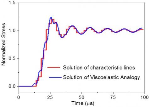
Figure 4 shows the stress history curve at the center position of the third layer, where the red step-like line is the exact solution obtained by the characteristic line method, and the blue curve represents the numerical solution obtained by Laplace numerical inversion, which almost coincides with the exact solution. Figure 5 compares the two solutions at the center position of the fifteenth layer. The third layer is the position near the action end, and the fifteenth layer is the position far from the action end. Figures 4 and 5 indicate that the numerical inversion method we used is accurate, and it also shows that the method of equivalent viscoelastic material based on periodic materials is appropriate.
Figure 4. Comparison of numerical and exact solutions in the center of layer 3
Figure 5. Comparison of numerical and exact solutions in the center of layer 15
Stress relaxation is a type of viscoelastic material. In this section, the characteristics of stress relaxation function in periodic materials are found by viscoelastic analogy method.
The characteristic time T (T=2 (h1+h2)/c2) is the time of one cycle of stress wave propagation; The thickness of a cycle is the characteristic length H (H=2 (h1+h2)). All original parameters and their dimensionless values in formula (17) are shown in Table 1. For the convenience of understanding, the parameters here are artificially selected, but without losing their generality.
Table 1. Physical properties of periodic material
|
Material Properties |
Original Values |
Normalized Value |
|
h1(m) |
0.0025 |
0.25 |
|
h2(m) |
0.0025 |
0.25 |
|
ρ1(kg/m3) |
8000 |
4 |
|
ρ2(kg/m3) |
2000 |
1 |
|
E1(GPa) |
200 |
4 |
|
E2(GPa) |
50 |
1 |
|
C1(m/s) |
5000 |
1 |
|
C2(m/s) |
5000 |
1 |
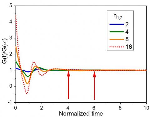
The original parameters are brought into formula (15) and the stress relaxation function curves of the periodic material are obtained using numerical Laplace inverse transform as shown in stress relaxation function curve of periodic materials as shown in Figure 6. With the increase of time, the stress relaxation function curve starts to decrease from the initial value and gradually stabilizes to the final value after several fluctuations. The relaxation curves of actual viscoelastic materials always monotonically decrease from the initial value and gradually approach the final value. This indicates that the periodic material exhibits a similar stress behavior as the actual viscoelastic material. In the relaxation image formula (17), the wave impedance and the thicknesses of the two materials are the two factors that affect the stress relaxation of the periodic material. Assuming that the thicknesses of the two materials are the same, varying the wave impedance ratio (η1,2) of the two materials yields different stress relaxation curves as shown in Figure 7. The larger the wave impedance ratio of the two materials, the more pronounced the relaxation characteristics exhibited by the periodic material. The physical property is that the closer the stiffness and density of the two materials are, especially when they are equal, i.e., when the wave impedance ratio is 1, the periodic material degrades to a material with no stress relaxation properties (linear elastic material) and vice versa.
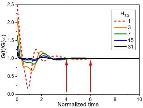
Assuming that the wave impedance ratio of the two materials is the same, changing the thickness ratio of the two materials(H1,2) can obtain the stress relaxation curves of periodic materials under different thickness ratios, as shown in Figure 7. From the figure, the larger the thickness ratio of the two materials, the smaller the relaxation characteristics of periodic materials. The physical property is that the larger the thickness ratio of the two materials, i.e., the more of one material and the less of the other, especially when the periodic material consists entirely of one material, the periodic material degenerates into one material (linear elastic material), and therefore does not have relaxation properties, and vice versa.
In addition, from Figures 7 and 8 show that the relaxation curve of the periodic material stabilizes after 4-6 times the characteristic time, and the relaxation properties gradually disappear. The physical property is that before the stress wave, the periodic material quickly (several times the characteristic time) degrades to a linear elastic material and loses the relaxation property.
Figure 6. Stress relaxation curves of periodic material
Figure 7. Effect of wave impedance ratio on relaxation curves of periodic material
Figure 8. Effect of thickness ratio on relaxation curve of periodic material
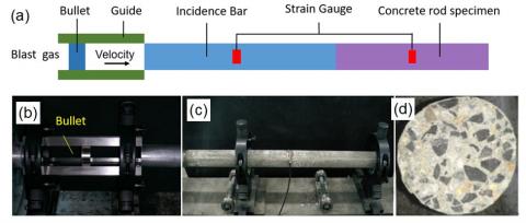
To further explore the stress wave propagation in concrete materials, we conducted impact compression experiments on SHPB or Kolsky rod [23] devices to characterize the high strain behavior of the materials. The Kolsky compression rod system generally consists of three major components: the pressure generation system (air gun and impact rods), the rod set (incident, transmissive, and absorbing rods), and the strain acquisition and recording system. In this study, the absorbing rods were removed to measure the propagation of stress waves in the rods.
The concrete rods are made of cement mortar and crushed stones. The cement mortar is #425 of China standard. The stones are natural rock or pebble made by mechanical crushing and screening, with particles size ranging from 1.75 mm to 4.75 mm. The Ratio of cement mortar and crushed stone are 1:3. The concrete specimens were removed from the molds 28 days after the completion of the pour.
The parameters of the concrete specimen are diameter D=74 mm, length L=1 m, mass M=10.2 kg, and density. It was found through testing that the average wave velocity of the concrete specimen was 4060 m/s and the elastic modulus was about 38 GPa. During the experiment, we designed a parallel device to improve the parallelism between the bullet and the incident bar, as shown in Figure 9.
As the stress attenuation analysis shows, the shorter the incident wavelength, the more obvious the stress wave attenuation. To observe significant stress attenuation phenomena, a shorter bullet was used to impact the SHPB incident bar to obtain a shorter incident wave. During the experiment, the stress wave attenuation process in the concrete specimen was observed, and the approximate stress attenuation curve in the concrete rod can be obtained by extracting the peak value of stress, as shown in Figure 10.
Based on the material parameters of the concrete specimen, it can be simplified as a periodic material composed of mortar and aggregate. The measured simplified periodic material parameters of concrete rod are listed in Table 2.
Figure 9. Experimental set up: (a) Schematic of SHPB experimental device; (b) Bullet slider; (c) Concrete rod; (d) Section image of concrete rod
Figure 10. Propagation and attenuation of stress wave in concrete specimen
Table 2. Properties of concrete rod
|
Material Properties |
Values |
Unit |
|
h1 |
0.003 |
m |
|
h2 |
0.003 |
m |
|
ρ1 |
2000 |
kg/m3 |
|
ρ2 |
2700 |
kg/m3 |
|
ρ |
2350 |
kg/m3 |
|
E1 |
25 |
GPa |
|
E2 |
80 |
GPa |
|
G(∞) |
38.09 |
GPa |
The stresses are normalized by initial value. Here, the initial stress value is extrapolated by fitting of peak values.
Finite element method is used in commercial code ABAQUS to simulate the wave propagation in concrete rod. Firstly, items, strike bullet, input bar and specimen, are established with the same size in experiment set up. The mesh size is about 1mm. There are 2,800,000 C3D8 elements in the model. The initial velocity of strike bullet is set 2 m/s. Contact property is surface to surface in Abaqus with no frictionless and hard normal contact function.
The simplified periodic material parameters are input into (18) and obtain stress history curves at different positions through Laplace numerical inverse transformation. By extracting the stress peak values, the stress attenuation curve in the periodic material can be obtained, as shown in Figure 11. The blue curve in the figure indicates the stress decay in concrete rods due to viscous factors calculated by analogy method. The red curve, calculated by the ABAQUS finite element method, represents the stress attenuation of concrete rods considering effects of geometric dispersion and kinematic depletion and kinematic energy. The green (square label) curve is the concrete rod stress attenuation curve measured in experiment.
The statistical results of maximum stress value measured at five times and ten times reflections. Results of seven concrete rods are listed in Table 3.
Figure 11. Comparison and analysis of the factors affecting stress attenuation in concrete specimens
Table 3. Statistical results of maximum stress value of experiments
|
Rod Number |
Stress at First Times (MPa) |
Stress at Five Times (MPa) |
Stress at Ten Times (MPa) |
|
#1 |
0.61 |
0.24 |
0.151 |
|
#2 |
0.52 |
0.30 |
0.132 |
|
#3 |
0.58 |
0.35 |
0.145 |
|
#4 |
0.73 |
0.45 |
0.143 |
|
#5 |
0.49 |
0.31 |
0.122 |
|
#6 |
0.62 |
0.36 |
0.155 |
|
#7 |
0.66 |
0.37 |
0.163 |
From Figure 10, the calculated results of the attenuation law of stress waves in concrete are consistent with the experimental values in trend, but the experimentally measured attenuation rate is slightly higher than the calculated attenuation rate. The main reasons for the differences are analyzed as follows:
Firstly, there is unavoidable friction between the concrete specimen and the SHPB support in the experiment, which consumes some energy. Friction involves complex contact problems, and it is difficult to obtain a true reflection through experiments and numerical calculations.
Secondly, in the numerical calculation, we treat the mortar and aggregate as elastic materials separately, but in fact, they are not completely elastic, they have certain viscosity, which leads to the calculated viscosity lower than the actual viscosity of concrete.
If the viscosities of mortar and aggregate are considered in their relaxation functions and the stress decay curves in concrete are further obtained by numerical transformations, the calculated results will be closer to the experimental results. However, if the viscosities of mortar and aggregate are considered in their relaxation functions, the Laplace numerical inversion method is invalid. A proper inversion method to deal the case will be developed in further study.
The stress wave propagation and attenuation laws in heterogeneous materials such as rock and concrete are investigated by equating these materials to periodic materials through the viscoelastic analogy method.
1) A numerical Laplace inversion code of Mathematica is developed to solve the functions of viscoelastic analogy method. The numerical Laplace inversion code is verified by the exact solutions based on the characteristic line theory.
2) Using the viscoelastic simulation method to equate a concrete bar to a periodic material, the attenuation law due to viscosity during the propagation of a stress wave in the equivalent periodic material is analyzed.
3) Comparison of experiments, ABAQUS finite element calculations and viscoelastic simulation methods for three stress attenuation laws shows that the comparison of the calculated results with the experimental results suggests that the causes affecting the stress attenuation are more complex. And the viscosity can partially explain the attenuation of stress waves in each periodic material.
This research is supported by the Open Fund Funding by National Engineering Laboratory for Applied Technology of Forestry & Ecology in South China (Grant number: 2023NFLY02) and the talent introduction project of Ningbo polytechnic (Grant number: RC202004).
|
σ |
Stress |
|
ε |
Strain |
|
ν |
Particle velocity |
|
ρ |
Density |
|
gi |
Stress relaxation function of layer i |
|
E |
Young's Modulus |
|
c |
Wave speed |
|
h1 |
Half thickness of layer 1 |
|
h2 |
Half thickness of layer 2 |
|
x |
Location along x axis direction |
|
T |
The characteristic time |
|
H |
The characteristic length |
|
A |
Stress load on the center of odder layer |
|
B |
Stress load on the center of even layer |
|
k |
The characteristic exponent |
|
p |
Frequency in Laplace field. |
|
G |
Stress relaxation of layered medium |
|
t |
Time |
|
D |
Dimeter of specimen |
|
L |
Length of specimen |
|
M |
Mass of specimen |
|
η1,2 |
The wave impedance ratio of two layers |
|
ω |
Half period of layered medium |
|
Φ |
Stress of response of layered medium |
|
s |
The characteristic exponent of Laplace transform |
|
σ |
Stress |
|
ε |
Strain |
|
ν |
Particle velocity |
Here shows the detail of application of numerical LaPlace transformation in Mathematica program.
First, physical properties of layered medium are assigned values.
Secondly, define the load function applied in the center of first layer.
σinc[t_]:=Piecewise[{{Sin[0.3927t],0<=t<=8},{0,8<t<=2000}}];
Sigma0[s_]:=LaplaceTransform[σinc[hihere],hihere,s]
Map001=Plot[σinc[t],{t,0,300},PlotRange->{-0.5,1.1},PlotStyle->{PointSize[5`],Hue[0]}]
INC[s_]:=Expand[Sigma0[s]]
Thirdly, input the stress function in form of Laplace field.
Set n=1; x=2 n ω. The stress function of (19) can be simplified as follows.
$\begin{aligned} & \bar{\sigma}[\mathrm{s}]:=\left(\frac{3.927 \times 10^7}{1.5421329 \times 10^7+1 . \times 10^8 \mathrm{~s}^2}+\frac{3.92699999989403 \times 10^7 \mathrm{e}^{-8 . s}}{1.5421329 \times 10^7+1 . \times 10^8 \mathrm{~s}^2}\right. \\ &\left.+\frac{734.6410206695457 \mathrm{e}^{-8 . \mathrm{s}} \mathrm{s}}{1.5421329 \times 10^7+1 . \times 10^8 \mathrm{~s}^2}\right)\left(\theta * \operatorname{Cosh}\left[2 * \mathrm{~s} \sqrt{\frac{\rho 1}{\mathrm{E} 1}} * \mathrm{~h} 1+2 * \mathrm{~s} \sqrt{\frac{\rho 2}{\mathrm{E} 2}} * \mathrm{~h} 2\right]-(\theta-1)\right. \\ &\left.* \operatorname{Cosh}\left[2 * \mathrm{~s} \sqrt{\frac{\rho 1}{\mathrm{E} 1}} * \mathrm{~h} 1-2 * \mathrm{~s} \sqrt{\frac{\rho 2}{\mathrm{E} 2}} * \mathrm{~h} 2\right]+\sqrt{}((\theta * \operatorname{Cosh}[2 * \mathrm{~s} \sqrt{\frac{\rho 1}{\mathrm{E} 1}} * \mathrm{~h} 1+2 * \mathrm{~s} \sqrt{\frac{\rho 2}{\mathrm{E} 2}} * \mathrm{~h} 2\right] \\ &\left.\left.-(\theta-1) * \operatorname{Cosh}\left[2 * \mathrm{~s} \sqrt{\frac{\rho 1}{\mathrm{E} 1}} * \mathrm{~h} 1-2 * \mathrm{~s} \sqrt{\frac{\rho 2}{\mathrm{E} 2}} * \mathrm{~h} 2\right]\right)+1\right) \sqrt{}((\theta * \operatorname{Cosh}\left[2 * \mathrm{~s} \sqrt{\frac{\rho 1}{\mathrm{E} 1}} * \mathrm{~h} 1+2\right. \\ &\left.\left.\left.\left.* \mathrm{~s} \sqrt{\frac{\rho 2}{\mathrm{E} 2}} * \mathrm{~h} 2\right]-(\theta-1) * \operatorname{Cosh}\left[2 * \mathrm{~s} \sqrt{\frac{\rho 1}{\mathrm{E} 1}} * \mathrm{~h} 1-2 * \mathrm{~s} \sqrt{\frac{\rho 2}{\mathrm{E} 2}} * \mathrm{~h} 2\right]\right)-1\right)\right)^{-x\sqrt{\frac{\rho}{4 . * \omega^2 * \rho}}}\end{aligned}$
Finally, define the Fourier Euler (FE) inversion method.
$\begin{aligned} & \mathrm{FE}[\mathrm{F\_}, \mathrm{t\_}, \mathrm{M\_}] \mathrm{]}:=\text { Module[\{a, prec3\}, prec3 } \\ & =\operatorname{Max}[M, \$ \text { MachinePrecision }] ; \xi 0=1 / 2 ; 1 \xi 1 \mathrm{M} \\ & =\text { Table[1, }\{M\}] ; \xi 2 \mathrm{M}=1 / 2^M ; \xi \mathrm{i}=\xi 2 \mathrm{M} ; l \xi \mathrm{Mp} 1 \mathrm{a} 2 \mathrm{Mm} 1 \\ & =\text { Reverse[Table[ } \xi \mathrm{i} \\ & \left.=\xi \mathrm{i}+\frac{1}{2^M} \frac{M!}{i!(M-i)!}\{\{i, 1, M-1\}]\right] ; \sqsupset 1 \xi \\ & =\operatorname{Join}[\{\xi 0\}, 1 \xi 1 \mathrm{M}, 1 \xi \mathrm{Mp} 1 \mathrm{a} 2 \mathrm{Mm} 1,\{\xi 2 \mathrm{M}\}] ; a \\ & =\text { SetPrecision }[M \log [10] / 3, \operatorname{prec} 3] ; \frac{\operatorname{Exp}[a]}{t} \operatorname{Sum}\left[(-1)^k 1 \xi[[k\right. \left.\left.+1]] \operatorname{Re}\left[F\left[\frac{a+I k \pi}{t}\right]\right],\{k, 0,2 M\}\right]\right] ; \\ & \end{aligned}$
The stress function in Laplace form can be inversed numerically by method above.
Here shows a sine load applied in the center of first layer. The peak value trend to attenuation with time increasement.
[1] Gopi, V., Swamy, K.K., Gopi, A.P., Narayana, V.L. (2020). Experimental study on shear behavior of reinforced concrete sandwich deep beam. Annales de Chimie - Science des Matériaux, 44(5): 301-309. https://doi.org/10.18280/acsm.440501
[2] Ma, C.L. (2021). Physical properties and durability of green fiber-reinforced concrete for road bridges. Annales de Chimie - Science des Matériaux, 2021, 45(2): 181-189. https://doi.org/10.18280/acsm.450211
[3] Zhao, Z., Wu, B., Zhang, Z., Yu, W. (2021). Impact strength characteristics of granite under combined dynamic and static loading conditions. Arabian Journal of Geosciences, 14: 1-7. https://doi.org/10.1007/s12517-020-06356-w
[4] Wang, J.G., Liang, S.F., Gao, Q.C., Li, X.L., Wang, L.N., Zhao, Y. (2018). Experimental study of jointed angles impact on energy transfer characteristics of simulated rock material. Journal of Central South University (Science and Technology), 49(5): 1237-1243. https://doi.org/10.11817/j.issn.1672-7207.2018.05.027
[5] Yu, X.L., Fu, Y.Q., Dong. X.L., Zhou, F.H., Ning, J.G., Xu, J.P. (2019). Full field DIC analysis of one-dimensional spall strength for concrete. Chinese Journal of Theoretical and Applied Mechanics, 51(4): 1064-1072. https://doi.org/10.6052/0459-1879-19-008
[6] Wu, X.T., Liao, L. (2017). Numerical simulation of stress wave attenuation in brittle material and spalling experiment design. Explosion and Shock Waves, 37(4): 705-711. https://doi.org/10.11883/1001-1455(2017)04-0705-07
[7] Li, X.P., Dong, Q., Liu, T.T., Huang, J.H. (2018). Research on propagation law of cylindrical stress wave in jointed rock mass under in-situ stress. Chinese Journal of Rock Mechanics and Engineering, 37(S1): 3121-3131. https://doi.org/10.13722/j.cnki.jrme.2017.1013
[8] Xu, H.F., Chen, X., Dong, L., Yang, Y.R. (2017). Equivalent elastic constants of rock containing pore fluid inclusions. Journal of Basic Science and Engineering, 25: 369-381. https://doi.org/10.16058/j.issn.1005-0930.2017.02.015
[9] Jin, J., Xu, H., Guo, Z., Liao, Z. (2022). An equivalent medium model of stress wave propagation through a three-dimensional geo-stressed rock. Arabian Journal of Geosciences, 15(14): 1236. https://doi.org/10.1007/s12517-022-10461-3
[10] Hu, W., Xu, M., Jiang, R., Zhang, F., Zhang, C., Deng, Z. (2021). Wave propagation in non-homogeneous centrosymmetric damping plate subjected to impact series. Journal of Vibration Engineering & Technologies, 9(8): 2183-2196. https://doi.org/10.1007/s42417-021-00355-1
[11] Liu, Y., Huang, Z.P., Wang, R. (1997). On the applicability of eshelby’ s equivalent inclusion method in nonlinear continumm mechanics. Acta Mechanica Sinica, 13(4): 506-512.
[12] Liu, D.L. (2021). Equivalent stiffness analysis of composite plate and shell structures based on quasi-periodic boundary condition. Dalian University of Technology, https://doi.org/10.26991/d.cnki.gdllu.2021.000006
[13] Huang, Z.M. (2023). Mechanics theories for composite materials. Acta Materiae Compositae Sinica, 40(6): 3090-3114. https://doi.org/10.13801/j.cnki.fhclxb.20230117.007
[14] Hegemier, G.A., Nayfeh, A.H. (1973). A continuum theory for wave propagation in laminated composites—case 1: Propagation normal to the laminates. Journal of Applied Mechanics, 40(2): 503-510. https://doi.org/10.1115/1.3423013
[15] Yuan, L., Miao, C., Xu, S., Xie, Y., Zhang, J., Li, Y., Gao, G., Wang, P. (2023). Stress-wave propagation in multilayered and density-graded viscoelastic medium. International Journal of Impact Engineering, 173: 104415. https://doi.org/10.1016/j.ijimpeng.2022.104415
[16] Ting, T.C.T., Mukunoki, I. (1979). A theory of viscoelastic analogy for wave propagation normal to the layering of a layered medium. Journal of Applied Mechanics, 46: 329-336. https://doi.org/10.1115/1.3424550
[17] Mukunoki, I., Ting, T.C.T. (1980). Transient wave propagation normal to the layering of a finite layered medium. International Journal of Solids and Structures, 16(3): 239-251. https://doi.org/10.1016/0020-7683(80)90077-3
[18] Ince, E.L. (1956). Ordinary Differential Equations. Courier Corporation. Dover Publishing, pp. 381-382.
[19] Brillouin, L. (1953). Wave Propagation in Periodic Structures: Electric Filters and Crystal Lattices. Dover Publishing, pp. 182.
[20] Jacquot, R.G., Steadman, J.W., Rhodine, C.N. (1983). The Gaver-Stehfest algorithm for approximate inversion of Laplace transforms. IEEE Circuits & Systems Magazine, 5(1): 4-8. https://doi.org/10.1109/MCAS.1983.6323897
[21] Cohen, A.M. (2007). Numerical Methods for Laplace Transform Inversion. Springer Science & Business Media.
[22] Abate, J., Valkó, P.P. (2004). Multi‐precision Laplace transform inversion. International Journal for Numerical Methods in Engineering, 60(5): 979-993. https://doi.org/org/10.1002/nme.995
[23] Chen, W.W., Song, B. (2010). Split Hopkinson (Kolsky) Bar: Design, Testing and Applications. Springer Science & Business Media.