D Rognatha Rao* | C Srinivas
© 2022 IIETA. This article is published by IIETA and is licensed under the CC BY 4.0 license (http://creativecommons.org/licenses/by/4.0/).
OPEN ACCESS
Micromachining techniques are now being used more frequently as a result of miniaturization. This technique has been supported by the requirement for material processing at an affordable cost and microatomic resolution in numerous sectors. Laser micromachining is a precise, non-contact method of machining that is used to create tiny, up to 500 m, components. The small elemental areas are the focus of laser ablation, which helps absorb a high amount of energy. In this micro-machining, metal removal rate and surface finish are represented by the deepness of the groove and the height of the recast layer. While machining, a layer called a recast layer forms on the work piece surface as a result of the tremendous heat generated, and this layer is damaging to the component's surface quality. For accurate applications, the recast layer must be as tiny as possible. As a result, the objective functions are the height of the recast layer and the deepness of the groove. Experiments designed by the DOE are used to generate empirical models. For each experimental run present in the matrix, the specified input parameter combination is set and the work piece is machined accordingly. The response surface methodology based on mathematical modeling and analysis of the machining properties of a pulsed Nd: YAG laser during micro-grooving operation on a work piece of Magnesium Silicon Alloy metal matrix composite is the focus of this research study. Initially, magnesium alloy AS21-SiC metal matrix composites are manufactured with Ultrasonic pro assisted stir casting. For the machined samples, the deepness of the groove and the height of recast layer will be measured by an optical measuring microscope. Consequently, the measured data is used by the GP to develop the mathematical models. In this work, an efficient GA-based genetic algorithm (NSGA-II) is applied to obtain the optimal parameters. As the chosen objectives are conflicting in nature, the problem is formulated as a multi-objective optimization problem.
genetic algorithm (NSGA-II), laser machining parameters, optimisation, and magnesium allay AS21-SiC, design expert
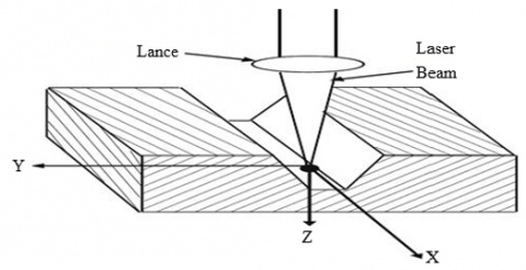
In this study, individual laser parameters are explored for their influence on Laser Micro Grooving processes, and process optimization is discussed in this paper. During laser grooving a blind cut is developed on the material, the schematic is shown in Figure 1. The present investigation aimed to explore some of the performance characteristics with the variation of particle size and volume percentage in AS21-SiC MMC along with some electrical machining parameters in Laser beam Micro-Machining
Figure 1. Cross sectional drawing of the desired micro groove
The experimentation is planned with the consideration of significant control variables as pulse power pulse frequency, assisted gas pressure and pulse width. The postulation of empirical models for deepness of machined micro groove and height of recast layer are also included.
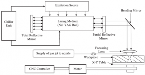
As well as this work formulates the Laser beam Micro-Machining of AS21-SiC explicitly as a multi-objective optimization problem to find the best machining parameters for the minimal recast layer height and maximum groove depth. The mathematical models for the selected machining responses are developed using response surface methodology (RSM). Further, these mathematical models are used in optimization to find the set of Pareto-optimal solutions. One of the efficient and widely used methods for generating Pareto frontier, an algorithm (NSGA-II) is applied to obtain the optimal parameters. Observed all parameters and selected some parameters for considering and get them optimised. Based on some investigations over this topic huge literature may be done and finalised the process parameters and optimisation technique. The overall methodology of present work is summarized as shown in Figure 2 below.
Figure 2. ND: YAG laser machine outline diagram
Utilizing the experimental test findings as produced from a predefined set of trials, the mathematical correlations between response, i.e., deviation half taper angle and deviation of depth with Nd: YAG laser micro-grooving process parameters have been established. The following steps have been taken to build a mathematical model based on RSM for correlating the groove depth and recast layer height as a function of the most popular laser machining process parameters as taken into account in the experimental design.
The multi-objective problem that is being optimised aims to increase the depth of the groove and minimise the height of the recast layer. Equations represent, respectively, the depth of the recast layer and the groove.
1.1 Literature survey
The quality of the laser cut is crucial to the laser cutting process. On the final product's quality, all cutting parameters may have a considerable impact. Cutting parameters are often modified and altered to deliver the desired cut quality. But doing this takes a lot of time and effort. Influence of the manufacturing parameters in laser melting on properties of an alloy described by Mauduit et al. [1]. Particulate reinforced metal matrix composites are described and studied in many researches [2-7]. Optical and conductive properties of composites and laser processing of composites are described [8]. Several attempts have also been made to model the LBM process. Although there has been a lot of foundational study [9, 10] in the domain of laser machining technology, there has been very little in the LMM. So, further research is still needed in the point of micromachining for optimal control of machining parameters. LMM is one of the most flexible and easiest to utilize. As a non-contact process, laser micro machining has the ability to be used on challenging materials and components either as part of a series of manufacturing process steps or in situ on completed parts. Advances in laser micro machining allow for fast, high-resolution,
accurate, reproducible processing. Windholz and Molian [11] described micro-machining of diamond by micro-second pulse Nd: YAG and nano-second pulse excimer lasers. Kovalenko et al. [12] reported micro drilling, micro cutting and micro milling of semiconductors with green laser. Elmes et al. [13] conclude that laser micromachining is the ideal technology for biomedical apparatus that requires improved speed and automation, such as a pin-based picolitre dispenser for taking thousands of genetic samples for huge parallel testing. Allen et al. [14] has fabricated inkjet nozzles of metal sheet by three different fabrication technique, i.e. micro-EDM, micro Drilling by using copper vapour laser machining and evaluated the characteristics of each technique while assessing the differences between. Drilling holes, however, is the key application in micro fabrication. Excimer laser removes only a thin layer of material and has small penetration depth, allowing precise control of the micro-drilling depth [15]. Although more number of research works are reported on laser drilling operation, research work on micro grooving operation using laser has not been reported so far. In several references, the applicability and superiority of the artificial neural network method of analysis has been reported [16, 17].
Process modeling and optimization are two important issues in LMM. The LBM process is characterized by a multiplicity of dynamically interacting process variables. Deepness of groove and height of recast layer are considered to be the important factors in predicting performance of Laser machining process. Dhara et al. [18] have adopted the artificial neural networks approach to optimize the machining parameter combination for the responses of deepness of groove and height of recast layer in laser micro-machining of die steel.
However, it is difficult to establish the relationship between LBM process parameters and responses because the process is too complex in nature. Therefore, response surface methodology (RSM) can be adopted for modeling and analysis using experimental data and studying the influence of various process parameters on responses [19]. Yildiz [20] proven the hybrid optimization approach's superiority over other strategies in terms of convergence speed and efficiency. Yusup et al. [21] For both conventional and modern machining, evolutionary strategies for optimising machining process parameters were considered. They observed evolutionary techniques while optimizing machining process parameters positively gives good results. Samantha and Chakraborty [22] showed the applicability and usefulness of evolutionary algorithms in improving unconventional machining processes' performance measures. Jain et al. [23] GA was utilized to optimize process parameters in advanced machining processes of the mechanical kind. As a result of these comprehensive investigations, evolutionary multi-objective optimization (EMO) approaches have become widely used in a variety of problem-solving tasks and have gotten a lot of attention from the multi-criterion optimization and decision-making communities [24]. Non-dominating sorting GA (NSGA-II) is one of the most widely used methods for generating the Pareto frontier. This algorithm ranks the individuals based on dominance. NSGA-II uses elitism and a phenotype crowd comparison operator that keeps diversity without specifying any additional parameters [25]. Deb et al. described a fast elitist non-dominated sorting genetic algorithm for multi-objective optimization: NSGA-II A new baseline algorithm for pareto multiobjective optimization [26, 27]. Its main advantage in solving multi-objective problems is that it leads the search toward the global Pareto front while maintaining diversity of the solution set along that front. A 7075 aluminum alloy matrix reinforced with 15 volume percent of SiCp were prepared by using liquid metallurgy route by Mohane t al. [28]. Optimization parameters of machining are described [29]. The Effect of evaporative pattern casting process parameters on the surface roughness of an alloy stated [30].
1.2 Nd: YAG laser machining system details for micro-grooving process
To generate complex machining operations such as profile cutting, grooving, shape cutting, marking, etc., The CNC pulsed Nd: YAG laser machining system is made up of several subsystems that operate in transverse electromagnetic mode, including the laser source and beam delivery unit, power supply unit, radio frequency (RF) Q-switch driver unit, cooling unit, and CNC controller for X, Y, and Z axis movement. The beam delivery system consists of a laser head, an RF Q switch, a safety shutter, a beam expander, and front and back mirrors. An Nd: YAG rod and a krypton arc lamp are arranged at two distinct focal points of an elliptical cavity in a laser head. Nd: YAG lasers use neodymium atoms as the lasing medium. The laser output is controlled by the current supplied to the krypton arc lamp by the main power supply unit. The cooling unit keeps the laser cavity, lamp, and Nd: YAG rod cold to avoid thermal damage.
Figure 3. Experimental setup of Nd: YAG laser beam machine
The CNC Nd: YAG laser machine is schematically represented in Figure 3. The Z-axis movement of the lens is controlled by the CNC Z-axis controller unit. Charge coupled device (CCD) cameras together with close circuit television (CCTV) are used for viewing the location of the work piece and also for checking the proper focusing condition of the surface of the work piece before laser machining for effective utilization of the place that is provided for fixing of the work piece. The crystal is excited by a krypton arc lamp. For amplification of light, optical feedback is provided with a rear mirror of 100% reflectivity and a front mirror of 80% reflectivity. Q-switching is a great way to get a very short pulse width and a high peak power of laser light from a low-power continuous wave (CW) laser. The RF Q-switch driver unit supplies an RF signal to the Q-switch for its operation. The laser is focused on the work area using a beam delivery mechanism. The CNC controller is made up of three axes: X, Y, and Z, as well as a controlling unit called accupos. Stepper motors are attached to each axis and connected to the accupos. This accupos unit can control the axis movement of the Nd: YAG laser beam.
Specifications of laser machine
|
Model |
JK300D |
|
Power at laser |
300W |
|
Typical power and work piece |
250w |
|
Maximum peak power |
16KW |
|
Max pulse energy |
35J |
|
Max frequency |
1000Hz |
|
Pulse width range |
0.2 – 5ms |
2.1 Conducting the experiments
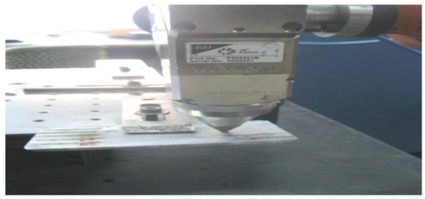
The current study's experimental setup is displayed in Figure 4. Figure 5 depicts the laser beam set up, the dielectric system, and the CNC system with the electronic circuits and controls for fixation of the work piece. Figure 4 displays the work piece setup and the LBM in a ready-to-start position. With offline CAD/CAM systems operating either three-axis flatbed systems for two-dimensional laser cutting or six-axis robots for three-dimensional laser cutting, the laser cutting process naturally leads to automation. The machine's running position is shown, as well as the spark and laser beam striking the work piece to create grooving. And no limitations on the cutting speed. Table 1 shows the possible ranges of process control variables offered by the machine tool manufacturer. These figures represent conditions in which there is no work piece breakage, no short circuits, and no cutting speed constraints. WEDM cuts manufactured materials to the jig's specifications, and finishing is done according to the nature of the job and the working environment. Wire a thin, single-strand metal wire and de-ionized water, which are used to carry electricity, are utilized in the electro thermal production process known as "EDM machining," which uses heat from electrical sparks to cut through metal. The feasible ranges of the process control variables, provided by the machine tool manufacturer, are listed in Table 1. These values correspond to the conditions under which there is no work piece break up, no short circuits, no other failure of the work material.
Figure 4. Experimentation of laser micro grooving during machining
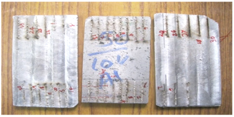
Figure 5. Work pieces after machining (grooving)
Table 1. Design of experimental matrix showing coded values
|
Exp. No. |
Pulse power(W) (A) |
Pulse frequency (Hz) (B) |
Gas pressure (Kg/cm3) (C) |
Pulse width (µm) (D) |
|
1. |
-1 |
-1 |
-1 |
-1 |
|
2. |
+1 |
-1 |
-1 |
-1 |
|
3. |
-1 |
+1 |
-1 |
-1 |
|
4. |
+1 |
+1 |
-1 |
-1 |
|
5. |
-1 |
-1 |
+1 |
-1 |
|
6. |
+1 |
-1 |
+1 |
-1 |
|
7. |
-1 |
+1 |
+1 |
-1 |
|
8. |
+1 |
+1 |
+1 |
-1 |
|
9. |
-1 |
-1 |
-1 |
+1 |
|
10. |
+1 |
-1 |
-1 |
+1 |
|
11. |
-1 |
+1 |
-1 |
+1 |
|
12. |
+1 |
+1 |
-1 |
+1 |
|
13. |
-1 |
-1 |
+1 |
+1 |
|
14. |
+1 |
-1 |
+1 |
+1 |
|
15. |
-1 |
+1 |
+1 |
+1 |
|
16. |
+1 |
+1 |
+1 |
+1 |
|
17. |
-2 |
0 |
0 |
0 |
|
18. |
+2 |
0 |
0 |
0 |
|
19. |
0 |
-2 |
0 |
0 |
|
20. |
0 |
+2 |
0 |
0 |
|
21. |
0 |
0 |
-2 |
0 |
|
22. |
0 |
0 |
+2 |
0 |
|
23. |
0 |
0 |
0 |
-2 |
|
24. |
0 |
0 |
0 |
+2 |
|
25. |
0 |
0 |
0 |
0 |
|
26. |
0 |
0 |
0 |
0 |
|
27. |
0 |
0 |
0 |
0 |
|
28. |
0 |
0 |
0 |
0 |
|
29. |
0 |
0 |
0 |
0 |
|
30. |
0 |
0 |
0 |
0 |
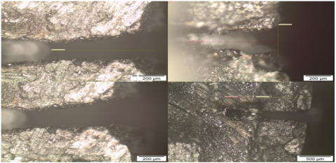
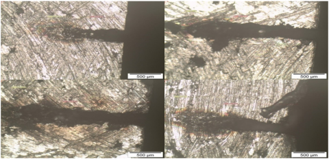
Figure 6. Microscopic images of machined work pieces that shows deepness of groove
Table 2. Design matrix four variable five level list of actual and coded values of the machining process parameters
|
S. No. |
Control factor |
Symbol |
Level |
Units |
||||
|
-2 (Lowest) |
-1 (low) |
0 (medium) |
1 (High) |
2 (highest) |
||||
|
1. |
Pulse power |
A |
210 |
220 |
230 |
240 |
250 |
W |
|
2. |
Pulse frequency |
B |
210 |
220 |
230 |
240 |
250 |
Hz |
|
3. |
Asst gas pressure |
C |
8 |
9 |
10 |
11 |
12 |
Kg/cm2 |
|
4. |
Pulse width |
D |
0.2 |
0.3 |
0.4 |
0.5 |
0.6 |
Ms |
2.1.1 Identify the process parameters
After marking and fixing the work piece on machine table machine power would be switched ON. The work item will then be grooved after a single laser pass. Four input variables have been chosen as a result of preliminary inquiry, namely
2.1.2 Conducting the experiments as per the design matrix and recording the responses
The machined work pieces are examined by an optical microscope by placing them on the table of the microscope, switching ON the light of the microscope, and connecting them to a computer that has microscope software installed. The lighting source emitted on the work piece would provide us with a microscopically clear view of the machined surfaces. The work piece's microscopically images are as shown in Figure 6.
2.1.3 Finding the control variables' upper and lower limits
The process variables' upper and lower bounds are determined. A factor's maximum and lower limits were coded as +2 and -2, respectively. Table 2 shows the selected process parameters together with their limit values.
2.2 Using design expert 7.1.4 to create mathematical models
In the present study, mathematical relationships between control variables and the output responses were developed using the RSM. For modeling the link between the process parameters and the output, RSM is a collection of advanced design experiments (DOE) approaches. Models with questionable response surface curvature are frequently improved using RSM. Two popular types of RSM used for experimenting are Box-Behnken Design (BBD) and Rotational Central Composite Design (RCCD). BBD is a capable and effective design. It is typically applied to nonsequential experiments. The RSM in a type BBD is carried out in this study with two objectives. Finding the ideal settings to reduce the dimensional inaccuracy is the first goal. The second is to look into how variables and responses interact in order to comprehend the system. The goal of constructing mathematical relationships is to link machining responses to cutting parameters, allowing for easier machining process optimization. The regression coefficients of the proposed models were calculated using Design Expert 7.1.4 statistical analysis software. Second order models were proposed due to the lower predictability of first order models for current models. The analysis of variance (ANOVA) was utilized to ensure that the proposed models were adequate.
2.2.1 Formulation of optimization problem
The mathematical relationships between response, i.e., deviation half taper angle and deviation of depth with Nd: YAG laser micro-grooving process parameters have been established utilizing the experimental test results as listed in Table 3 obtained from a planned set of experiments. Mathematical model based on RSM for correlating the groove depth and recast layer height as a function of the most common laser machining process parameters as considered in the experimental design have been established through the following.
In the process of optimization, the aim is to maximize the deepness of groove and minimize height of recast layer which forms the multi objective problem. Equations represent the deepness of groove and recast layer respectively. The complexities of the models were reduced by applying the back elimination procedure. The final equations, after eliminating the insignificant terms, as:
2.2.2 In terms of coded factors - Deepness of the groove
Deepness of Groove=+0.058+0.020×A+6.567E-003×B+3.383E-003×C-6.167E-004×D+5.800E-003×A×B+5.200E-003×A×C-3.400E-003×A×D-5.000E-005×B×C-5.850E 003×B×D+5.500E-004×C×D+3.650E-003×A2-6.100E-003×B2+8.500E-4×C2+7.500E-004× D2 (2.1)
2.2.3 In terms of coded factors-height of recast layer
Height of Recast Layer =+0.045+0.011×A+0.022×B+2.906E-003×C-3.639E-003×D+4.782E-0×A×B+1.818E-003×A×C+4.583E-003×A×D+7.417E-003B×C+2.282E-003×B×D-3.482E-003×C×D-4.186E-003×A2+6.714E-003×B2+4.137E-004×C2-9.863E-004× D2 (2.2)
In the above equations A, B, C, and D, represents logarithmic transformation of machining parameters that is pulse power, pulse frequency, gas pressure and pulse width. In the Eqns. (2.1) and (2.2), A, B, C, and D represent the logarithmic transformations of control factors is pulse power, pulse frequency, gas pressure and pulse width respectively and they are given below:
$x_1=\frac{\ln \left(X_1\right)-\ln (9)}{\ln (11)-\ln (9)} ; x_2=\frac{\ln \left(X_2\right)-\ln (30)}{\ln (35)-\ln (30)}$;
$x_3=\frac{\ln \left(X_3\right)-\ln (5)}{\ln (7)-\ln (5)} ; x_4=\frac{\ln \left(X_4\right)-\ln (5)}{\ln (6)-\ln (5)}$
The above relations are obtained from the following transformation equation:
$x=\frac{\ln \left(X_n\right)-\ln \left(X_{n 0}\right)}{\ln \left(X_{n 1}\right)-\ln \left(X_{n 0}\right)}$
where, x is the coded value of any factor corresponding to its natural value Xn; Xn1 is the natural value of the factor.
2.3 Analysis of variance (ANOVA)
The Model F-value of 9.32 indicates that the model is statistically significant. Due to noise, there is only a 0.01 percent chance that a "Model F-Value" this large will occur. Model terms are significant when "Prob > F" is less than 0.0500. A and B are important model terms in this scenario. The model terms are not important if the value is bigger than 0.1000. Tables 4 and 5 exhibit the ANOVA statistics for deepness of groove and height of recast layer, respectively.
2.3.1 ANOVA for groove depth
The Model F-value of 9.32 in Table 4 indicates that the model is significant. Due to noise, there is only a 0.01 percent chance that a "Model F-Value" this large will occur. Model terms are significant when "Prob > F" is less than 0.0500. A and B are important model terms in this scenario. The model terms are not important if the value is bigger than 0.1000. If there are a lot of minor model terms. The "Lack of Fit F-value" of 1.39 indicates that the lack of fit has no bearing on the pure error. A large "Lack of Fit F-value" has a 37.53 percent chance of occurring owing to noise.
Table 3. Design of experimental matrix showing observed responses
|
Ex.No. |
Pulse power (W) |
Pulse frequency (Hz) |
Gas pressure (Kg/Cm) |
Pulse width (Ms) |
Deepness of groove (mm) |
Height of recast layer (mm) |
|
1 |
240 |
220 |
11 |
0.5 |
0.0705 |
0.0359 |
|
2 |
220 |
220 |
9 |
0.5 |
0.0525 |
0.0298 |
|
3 |
230 |
230 |
10 |
0.4 |
0.0651 |
0.0397 |
|
4 |
220 |
240 |
11 |
0.5 |
0.0503 |
0.0492 |
|
5 |
220 |
220 |
11 |
0.3 |
0.0492 |
0.0321 |
|
6 |
230 |
230 |
10 |
0.4 |
0.0552 |
0.0405 |
|
7 |
240 |
220 |
9 |
0.3 |
0.0657 |
0.0427 |
|
8 |
240 |
240 |
11 |
0.3 |
0.0798 |
0.0699 |
|
9 |
220 |
240 |
9 |
0.3 |
0.0532 |
0.0527 |
|
10 |
240 |
240 |
9 |
0.5 |
0.0687 |
0.06523 |
|
11 |
220 |
240 |
11 |
0.3 |
0.0502 |
0.0578 |
|
12 |
220 |
240 |
9 |
0.5 |
0.0442 |
0.0469 |
|
13 |
220 |
220 |
9 |
0.3 |
0.0421 |
0.0321 |
|
14 |
230 |
230 |
10 |
0.4 |
0.0553 |
0.0416 |
|
15 |
240 |
240 |
11 |
0.5 |
0.0695 |
0.0689 |
|
16 |
240 |
220 |
9 |
0.5 |
0.0557 |
0.0378 |
|
17 |
230 |
230 |
10 |
0.4 |
0.0553 |
0.0497 |
|
18 |
240 |
240 |
9 |
0.3 |
0.0696 |
0.0547 |
|
19 |
220 |
220 |
11 |
0.5 |
0.0461 |
0.0302 |
|
20 |
240 |
220 |
11 |
0.3 |
0.0645 |
0.0408 |
|
21 |
230 |
230 |
10 |
0.4 |
0.0552 |
0.0501 |
|
22 |
250 |
230 |
10 |
0.4 |
0.0799 |
0.0529 |
|
23 |
230 |
250 |
10 |
0.4 |
0.0602 |
0.0695 |
|
24 |
230 |
230 |
10 |
0.2 |
0.0548 |
0.0493 |
|
25 |
230 |
230 |
12 |
0.4 |
0.0603 |
0.0475 |
|
26 |
230 |
230 |
8 |
0.4 |
0.0542 |
0.0415 |
|
27 |
230 |
230 |
10 |
0.4 |
0.0605 |
0.0513 |
|
28 |
210 |
230 |
10 |
0.4 |
0.0402 |
0.0269 |
|
29 |
230 |
230 |
10 |
0.6 |
0.0595 |
0.0369 |
|
30 |
230 |
210 |
10 |
0.4 |
0.0404 |
0.0321 |
Table 4. Analysis of variance table for response surface quadratic model
|
Source |
Sum of squares |
Degrees of freedom |
Mean square |
F-value |
P-value |
|
A-pulse power |
2.313E-003 |
1 |
2.313E-003 |
105.80 |
<0.0001 |
|
B-frequency |
2.587E-004 |
1 |
2.587E-004 |
11.84 |
0.0036 |
|
C-pressure |
6.868E-005 |
1 |
6.868E-005 |
3.14 |
0.0966 |
|
D-width |
2.282E-006 |
1 |
2.282E-006 |
0.10 |
0.7511 |
|
AB |
3.364E-005 |
1 |
3.364E-005 |
1.54 |
0.2338 |
|
AC |
2.704E-005 |
1 |
2.704E-005 |
1.24 |
0.2836 |
|
AD |
1.156E-005 |
1 |
1.156E-005 |
0.53 |
0.4783 |
|
BC |
2.500E-009 |
1 |
2.500E-009 |
1.144 |
0.9916 |
|
BD |
3.422E-005 |
1 |
3.422E-005 |
1.57 |
0.2300 |
|
CD |
3.025E-007 |
1 |
3.025E-007 |
0.014 |
0.9079 |
|
A2 |
2.284E-005 |
1 |
2.284E-005 |
1.04 |
0.3229 |
|
B2 |
6.379E-005 |
1 |
6.379E-005 |
2.92 |
0.1082 |
|
C2 |
1.239E-006 |
1 |
1.239E-006 |
0.057 |
0.8151 |
|
D2 |
9.643E-007 |
1 |
9.643E-007 |
0.044 |
0.8365 |
|
Residual |
3.279E-004 |
15 |
2.186E-005 |
|
|
|
Lack of Fit |
2.413E-004 |
10 |
2.413E-005 |
1.39 |
0.3753 |
|
Pure Error |
8.659E-005 |
5 |
1.732E-005 |
|
|
|
Cor Total |
3.181E-003 |
29 |
|
|
|
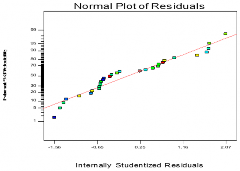
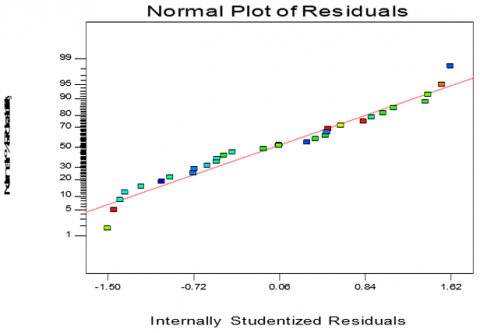
Figure 7. Normal plots of residuals
From the notation the "Pred R-Squared" of 0.5238 is not as close to the "Adj R-Squared" of 0.8007 as one might normally expect. This may indicate a large block effect or a possible problem with the model and/or data.
Model reduction, response transformation, outliers, and other factors should all be considered. The signal-to-noise ratio is measured using "Adeq Precision." It is preferable to have a ratio of more than four. Your signal-to-noise ratio of 11.877 suggests a good signal.
The design space can be navigated using this concept.
|
Std. Dev. |
4.675E-003 |
|
R-Squared |
0.8969 |
|
Mean |
0.058 |
|
Adj R-Squared |
0.8007 |
|
C.V. % |
8.12 |
|
PredR-Squared |
0.5238 |
|
PRESS |
1.515E-003 |
|
Adeq Precision |
11.877 |
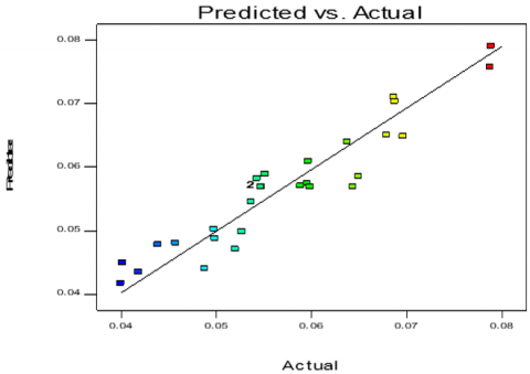
After all models is significant normal% of probability plots are represented in graphical as shown in Figure 7. As well as a graph was drawn in between actual values and predicted values to check the fitness of the given values as shown in Figure 8.
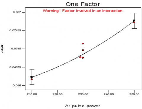
The individual influence of pulse power on groove depth is seen in Figure 9. It shows that as the pulse power grows, so does the depth of the groove. The depth of the groove deepens as the pulse power increases, according to the results of the experiments. Figure 10 shows that pulse frequency increases the deepness of the groove also increases on the other hand upto certain range then decreases.
Figure 8. Actual values Vs predicted values
Figure 9. Effect of pulse power on deepness of groove
Figure 10. Effect of frequency on deepness of groove
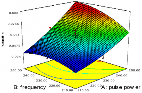
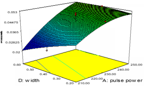
Figure 11. Effect of pulse frequency and pulse power on deepness of groove
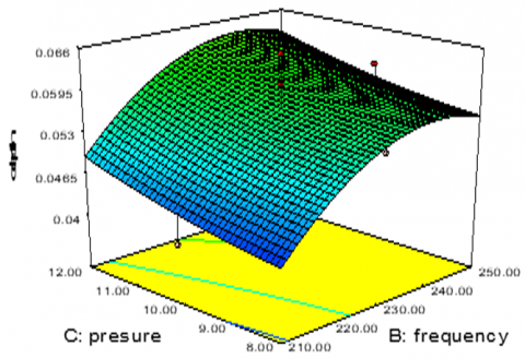
Figure 12. Effect of gas pressure and pulse frequency on deepness of groove
The interaction effect of pulse power and pulse frequency on deepness of groove is as shown in Figure 11. At a constant pulse frequency pulse power is directly proportional to deepness of the groove.
Comparatively at low value of pulse power, pulse frequency has parabolic effect on deepness of the groove. Even if the pulse frequency is increased or decreased, the groove depth is not impacted. On the other hand, when the pulse power is high, the depth of the groove deepens as the pulse frequency rises.
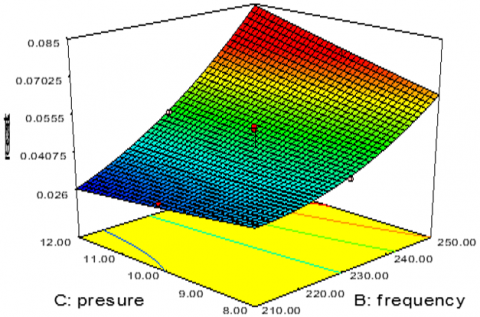
Figure 12 depicts the interaction effect of gas pressure and pulse frequency on groove depth. When the effect of assist gas pressure increases, the depth of the groove reduces as the pulse frequency increases. However, when the frequency of the pulse increases, the depth of the groove deepens and subsequently declines. We can see that increasing the pulse frequency has a considerably greater influence on groove depth.
2.3.2 ANOVA for recast layer
In the Table 5 the F-value of 13.46 for the model indicates that it is significant. Due to noise, there is only a 0.01 percent chance that a "Model F-Value" this large will occur.
The "Lack of Fit F-value" of 0.57 indicates that the lack of fit has no bearing on the pure error. There's a 78.70 percent likelihood that a significant "Lack of Fit F-value" is caused by noise.
|
Std. Dev. |
4.578E-003 |
|
R-Squared |
0.9263 |
|
Mean |
0.046 |
|
Adj R-Squared |
0.8575 |
|
C.V. % |
9.98 |
|
Pred R-Squared |
0.7236 |
|
PRESS 1. |
179E-003 |
|
Adeq Precision |
14.936 |
Table 5. Analysis of variance table for response surface quadratic model
|
Source |
Sum of squares |
Degrees of freedom |
Mean square |
F-value |
P-value |
|
A-pulse power |
7.835E-004 |
1 |
7.835E-004 |
37.39 |
<0.0001 |
|
B-frequency |
2.789E-003 |
1 |
2.789E-003 |
133.10 |
<0.0001 |
|
C-pressure |
5.066E-005 |
1 |
5.066E-005 |
2.42 |
0.1408 |
|
D-width |
7.946E-005 |
1 |
7.946E-005 |
3.79 |
0.0705 |
|
AB |
2.287E-005 |
1 |
2.287E-005 |
1.09 |
0.3127 |
|
AC |
3.303E-006 |
1 |
3.303E-006 |
0.16 |
0.6969 |
|
AD |
2.100E-005 |
1 |
2.100E-005 |
1.00 |
0.3327 |
|
BC |
5.502E-005 |
1 |
5.502E-005 |
2.63 |
0.1260 |
|
BD |
5.210E-006 |
1 |
5.210E-006 |
0.25 |
0.6253 |
|
CD |
1.213E-005 |
1 |
1.213E-005 |
0.58 |
0.4586 |
|
A2 |
3.004E-005 |
1 |
3.004E-005 |
1.43 |
0.2498 |
|
B2 |
7.727E-005 |
1 |
7.727E-005 |
3.69 |
0.0740 |
|
C2 |
2.935E-007 |
1 |
2.935E-007 |
0.014 |
0.9074 |
|
D2 |
1.667E-006 |
1 |
1.667E-006 |
0.080 |
0.7817 |
|
Residual |
3.143E-004 |
15 |
2.096E-005 |
|
|
|
Lack of Fit |
1.680E-004 |
10 |
1.680E-005 |
0.57 |
0.7870 |
|
Pure Error |
1.463E-004 |
5 |
2.926E-005 |
|
|
|
Cor Total |
4.263E-003 |
29 |
|
|
|
Figure 13. Normal plot of residuals of recast layer
Figure 14. Graph in terms of actual values vs. predicted
Figure 15. Effect of pulse frequency and pulse power on recast layer
The "Pred R-Squared" of 0.7236 is in reasonable agreement with the "Adj R-Squared" of 0.8575, as seen in the above notation. The signal-to-noise ratio is measured using "Adeq Precision." It is preferable to have a ratio of more than four. Your signal-to-noise ratio of 14.936 suggests a good signal. This model can be used to find your way through the design world.
Figure 13 shows normal percent of probability graphs once all models are significant. In contrast, in Figure 14, a graph was formed between actual and anticipated values.
Figure 15 depicts the effect of pulse power and pulse frequency on the height of the recast layer. At varying inputs of pulse power, the height of the recast layer grows as the pulse frequency increases; at the same time, the height of the recast layer increases as the pulse power increases. This phenomenon demonstrates that the pulse frequency has a greater impact on the recast layer than the pulse power.
Figure 16 depicts the effect of pulse width and pulse power on the height of the recast layer. We can see that when pulse width rises, the height of the recast layer likewise increases, and as pulse power increases, the height of the recast layer also increases. On the recast layer, we can see that pulse power is more effective than pulse width.
Figure 16. Effect of pulse width and pulse power on recast layer
Figure 17 depicts the effect of gas pressure and pulse frequency on the recast layer. When the pulse frequency is increased, the height of the recast layer increases with a decrease in gas pressure, but there is no adverse effect on the recast layer when the air pressure is increased.
Figure 17. Effect of air pressure and pulse frequency on recast layer
In quadratic model the F-value of deepness of groove is 1.39 and for the height of recast layer 0.57, shows the quadratic model is significant. The F-value and P-values for linear and cubic models is as shown in Table 6.
Table 6. Result of analysis of variance of developed model
|
Source |
Deepness of groove |
Height of recast layer |
||
|
F-value |
P-value |
F-value |
P-value |
|
|
Linear |
1.30 |
0.415 |
0.71 |
0.7375 |
|
Model |
9.32 |
0.0001 |
13.46 |
0.0001 |
|
Quadratic |
1.39 |
0.3753 |
0.57 |
0.7870 |
|
Cubic |
4.80 |
0.0685 |
0.47 |
0.6477 |
|
Lack of fit |
1.39 |
0.3753 |
0.57 |
0.7870 |
The data are plotted and also presented in the format of table and graphical methods. The experimental data are examined and analyzed in great details. With NSGA-II, optimal parameter sets are computed using response surface approach. The contribution of parameters is determined using analysis of variance. The validity of the ideal outcomes is demonstrated by a confirmation result. The choice of a solution has to be made based on production requirements. The optimal values of the input variables and their corresponding objective function values are listed in Table 7.
Table 7. Optimal values obtained through NSGA-II of the input variables and their objective function values
|
S.No. |
Pulse power (W) |
Pulse frequency (Hz) |
Assisted gas pressure (Kg/cm2) |
Pulse width (ms) |
Deepness of groove (mm) |
Height of recast layer (mm) |
|
1 |
210.7657 |
222.211 |
11.92756 |
0.200092 |
2.310746 |
0.050708 |
|
2 |
210.009 |
249.664 |
10.34353 |
0.200723 |
1.670608 |
0.040839 |
|
3 |
210.0025 |
249.8956 |
10.08455 |
0.200348 |
1.620358 |
0.039515 |
|
4 |
210.0134 |
241.1871 |
11.99243 |
0.200075 |
2.006495 |
0.048514 |
|
5 |
249.9972 |
218.8558 |
8.002752 |
0.59681 |
0.859658 |
0.021433 |
|
6 |
210.0199 |
249.8648 |
9.564685 |
0.200129 |
1.510591 |
0.036566 |
|
7 |
210.0181 |
236.4169 |
11.98223 |
0.200131 |
2.068817 |
0.048882 |
|
8 |
210.0014 |
249.5055 |
9.785729 |
0.200194 |
1.559961 |
0.03783 |
|
9 |
210.0344 |
249.9703 |
8.625887 |
0.200134 |
1.27043 |
0.030373 |
|
10 |
210.0528 |
249.723 |
9.787448 |
0.212467 |
1.553616 |
0.037107 |
|
11 |
210.0627 |
212.2491 |
11.99163 |
0.200197 |
2.591133 |
0.053919 |
|
12 |
249.9954 |
214.0244 |
8.710488 |
0.599913 |
1.142144 |
0.027227 |
|
13 |
210.2102 |
249.8255 |
9.100176 |
0.200108 |
1.399756 |
0.033622 |
|
14 |
210.0485 |
249.871 |
9.426269 |
0.200095 |
1.478824 |
0.035724 |
|
15 |
210.0648 |
249.9518 |
10.95623 |
0.200021 |
1.77451 |
0.04386 |
|
16 |
249.9954 |
210.7741 |
8.713378 |
0.599982 |
1.202755 |
0.028692 |
|
17 |
249.9981 |
215.1966 |
8.688335 |
0.599993 |
1.115994 |
0.026618 |
|
18 |
249.9891 |
237.0346 |
8.004148 |
0.599948 |
0.738663 |
0.016951 |
|
19 |
249.9663 |
210.2643 |
8.750101 |
0.598289 |
1.224507 |
0.029116 |
|
20 |
210.009 |
249.922 |
10.8878 |
0.204209 |
1.761492 |
0.04326 |
|
21 |
210.018 |
249.9264 |
8.730183 |
0.200309 |
1.299882 |
0.031109 |
|
22 |
249.9943 |
242.141 |
8.000059 |
0.599889 |
0.733183 |
0.016157 |
|
23 |
210.0013 |
248.3517 |
8.372686 |
0.200014 |
1.191695 |
0.028234 |
|
24 |
249.9895 |
210.6772 |
8.251802 |
0.599998 |
1.059454 |
0.026083 |
|
25 |
249.966 |
222.4058 |
8.000406 |
0.599543 |
0.820953 |
0.020331 |
|
26 |
210.7674 |
236.3836 |
11.98204 |
0.200131 |
2.062748 |
0.048684 |
|
27 |
210.0048 |
249.8245 |
9.058958 |
0.200122 |
1.388371 |
0.03337 |
|
28 |
249.7002 |
214.9657 |
8.016298 |
0.599991 |
0.916903 |
0.022947 |
|
29 |
210.0123 |
210.1892 |
11.99314 |
0.596043 |
3.071835 |
0.057376 |
|
30 |
210.7092 |
249.6414 |
8.172987 |
0.200131 |
1.13535 |
0.026821 |
|
31 |
210.7878 |
249.9111 |
11.92756 |
0.200196 |
1.907289 |
0.047718 |
|
32 |
249.9873 |
214.0653 |
8.035525 |
0.599975 |
0.93204 |
0.023371 |
|
33 |
249.9839 |
210.8045 |
8.139911 |
0.599976 |
1.019442 |
0.025338 |
|
34 |
210.0013 |
249.7235 |
9.875699 |
0.200057 |
1.578539 |
0.038369 |
|
35 |
210.001 |
233.5723 |
11.99773 |
0.200005 |
2.115064 |
0.049292 |
|
36 |
210.0027 |
214.2002 |
11.99896 |
0.20014 |
2.53785 |
0.053371 |
|
37 |
210.582 |
210.7828 |
11.96816 |
0.579998 |
3.010161 |
0.056339 |
|
38 |
249.5073 |
212.9607 |
8.713378 |
0.599916 |
1.170274 |
0.027782 |
|
39 |
210.0096 |
212.6306 |
11.98562 |
0.599268 |
2.961924 |
0.055746 |
|
40 |
249.9839 |
214.4303 |
8.145487 |
0.599975 |
0.963394 |
0.023901 |
|
41 |
210.094 |
213.1367 |
11.96816 |
0.57951 |
2.922053 |
0.055025 |
|
42 |
249.9895 |
236.2968 |
8.251802 |
0.596663 |
0.803108 |
0.01822 |
|
43 |
210.0062 |
218.7938 |
11.99672 |
0.200242 |
2.416165 |
0.052077 |
|
44 |
210.0014 |
249.1198 |
8.808909 |
0.200192 |
1.321282 |
0.031565 |
|
45 |
210.1036 |
211.0404 |
11.99927 |
0.59982 |
3.033379 |
0.05683 |
|
46 |
210.0528 |
249.7688 |
9.787448 |
0.214816 |
1.552304 |
0.036978 |
|
47 |
210.0013 |
249.7235 |
9.913887 |
0.200062 |
1.586484 |
0.038583 |
|
48 |
210.8063 |
221.3721 |
11.99581 |
0.200226 |
2.342294 |
0.051217 |
|
49 |
249.9687 |
216.6826 |
8.011403 |
0.599918 |
0.888277 |
0.022261 |
|
50 |
249.9895 |
210.6772 |
8.251802 |
0.599998 |
1.059454 |
0.026083 |
|
51 |
249.9839 |
210.8045 |
8.16757 |
0.599976 |
1.028906 |
0.025511 |
|
52 |
210.0012 |
249.9151 |
9.16406 |
0.200094 |
1.415078 |
0.034075 |
|
53 |
210.0218 |
221.7296 |
11.59395 |
0.200018 |
2.264957 |
0.04931 |
|
54 |
210.0126 |
247.214 |
11.99902 |
0.200005 |
1.942509 |
0.048252 |
|
55 |
210.732 |
249.9322 |
10.63538 |
0.219361 |
1.710256 |
0.040962 |
|
56 |
249.9687 |
234.8126 |
8.014626 |
0.599918 |
0.747281 |
0.017404 |
|
57 |
210.205 |
212.7821 |
11.98218 |
0.202428 |
2.574921 |
0.053602 |
|
58 |
210.0065 |
249.8966 |
10.24855 |
0.201414 |
1.651524 |
0.040315 |
|
59 |
249.4754 |
210.6624 |
8.002235 |
0.599559 |
0.981969 |
0.02458 |
|
60 |
210.0012 |
249.9151 |
9.185439 |
0.200059 |
1.420441 |
0.034215 |
|
61 |
210.0014 |
249.5055 |
9.783211 |
0.200063 |
1.559487 |
0.037823 |
|
62 |
210.0121 |
249.9329 |
8.906801 |
0.200029 |
1.348454 |
0.032361 |
|
63 |
210.0653 |
249.5856 |
9.303127 |
0.20003 |
1.449859 |
0.034926 |
|
64 |
210.0023 |
210.0022 |
11.99164 |
0.20021 |
2.659919 |
0.054685 |
|
65 |
210.0025 |
249.8959 |
10.22068 |
0.20538 |
1.644092 |
0.03991 |
|
66 |
210.0036 |
249.1216 |
8.885356 |
0.200038 |
1.342381 |
0.032108 |
|
67 |
249.8794 |
221.3033 |
8.034429 |
0.599999 |
0.843263 |
0.020873 |
|
68 |
210.0112 |
249.9329 |
11.4259 |
0.218886 |
1.833854 |
0.044613 |
|
69 |
210.0008 |
249.9816 |
11.73381 |
0.200475 |
1.885147 |
0.047143 |
|
70 |
210.8507 |
210.7828 |
11.96816 |
0.579998 |
3.001211 |
0.056206 |
|
71 |
249.4754 |
210.6871 |
8.015484 |
0.599559 |
0.98629 |
0.024655 |
|
72 |
210.0311 |
249.9111 |
11.92756 |
0.200108 |
1.910111 |
0.047916 |
|
73 |
210.7629 |
218.8851 |
11.99338 |
0.200473 |
2.401768 |
0.051812 |
|
74 |
210.0123 |
210.1892 |
11.99314 |
0.596043 |
3.071835 |
0.057376 |
|
75 |
210.1445 |
234.7456 |
11.99243 |
0.200075 |
2.094342 |
0.049081 |
|
76 |
249.8266 |
241.2541 |
8.014626 |
0.599918 |
0.73754 |
0.016359 |
|
77 |
210.1557 |
216.8298 |
11.99709 |
0.2 |
2.463572 |
0.052564 |
|
78 |
210.1036 |
211.0404 |
11.99948 |
0.59982 |
3.033423 |
0.056831 |
|
79 |
210.0034 |
249.9993 |
10.69499 |
0.200013 |
1.731724 |
0.042652 |
|
80 |
210.0077 |
249.8239 |
8.702315 |
0.201364 |
1.291353 |
0.030838 |
|
81 |
210.0485 |
249.9225 |
8.972773 |
0.200108 |
1.366101 |
0.032801 |
|
82 |
210.205 |
213.3747 |
11.96806 |
0.570347 |
2.902937 |
0.054693 |
|
83 |
210.0112 |
249.9329 |
11.4259 |
0.215233 |
1.835842 |
0.04485 |
|
84 |
210.0112 |
249.9322 |
10.63538 |
0.21647 |
1.712976 |
0.041285 |
|
85 |
210.0054 |
214.2252 |
11.91599 |
0.200208 |
2.519464 |
0.052919 |
|
86 |
210.0077 |
221.1555 |
11.99782 |
0.200005 |
2.359081 |
0.051512 |
|
87 |
210.0485 |
249.871 |
9.426269 |
0.200095 |
1.478824 |
0.035724 |
|
88 |
210.0134 |
241.2864 |
11.93546 |
0.200081 |
1.99718 |
0.048271 |
|
89 |
210.0091 |
249.9531 |
9.538919 |
0.204219 |
1.502444 |
0.03617 |
|
90 |
249.9873 |
213.1771 |
8.035525 |
0.599995 |
0.945255 |
0.023716 |
|
91 |
210.651 |
221.387 |
11.70816 |
0.200226 |
2.287587 |
0.049804 |
|
92 |
249.9895 |
236.2968 |
8.251802 |
0.596663 |
0.803108 |
0.01822 |
|
93 |
210.0025 |
249.8956 |
10.05825 |
0.200348 |
1.61514 |
0.039373 |
|
94 |
210.0648 |
249.9518 |
10.95623 |
0.200021 |
1.77451 |
0.04386 |
|
95 |
210.0124 |
211.051 |
11.97076 |
0.200038 |
2.622739 |
0.054216 |
|
96 |
210.0032 |
249.9993 |
10.6916 |
0.200128 |
1.731087 |
0.042628 |
|
97 |
210.7657 |
222.211 |
11.92756 |
0.200092 |
2.310746 |
0.050708 |
|
98 |
210.0371 |
216.8298 |
11.99709 |
0.200029 |
2.465562 |
0.052598 |
|
99 |
210.0045 |
249.8043 |
8.535565 |
0.200958 |
1.24323 |
0.029642 |
|
100 |
210.0095 |
212.6306 |
11.9724 |
0.598787 |
2.958856 |
0.055685 |
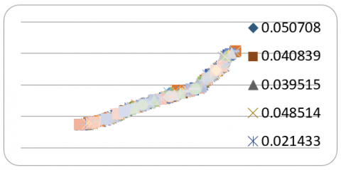
Figure 18. Graphical representations of optimal pareto front values
3.1 Pareto optimal values obtained from NSGA-II
The deepness of the groove and the height of the recast layer were optimised using the non-dominating sorting genetic algorithm-II, a multi-objective optimization method. Table 7 illustrates the Pareto-optimal set of 100 solutions that was obtained.
The proposed algorithm was implemented using VC++ and run on a Core 2 Duo system. The algorithm was run for ten times to get more number of points in the Pareto-optimal front. The pareto-solution set is obtained and the final set of solutions is the non-dominated solution set obtained for the optimization problem. The objective function values of The Pareto-optimal front obtained is shown in Figure 18. As it can be observed from the graph, no solution in the front is better than any other as they are non-dominated solutions.
The Nd: YAG laser machining system has the capability to perform successful precision micro-grooving operations on magnesium composite. The process parameters can be optimally controlled to minimize the height of the recast layer and maximize the deepness of laser micro-grooves. From the investigation during the machining of AS21-SiC by the Nd: YAG laser, the following outcomes can be obtained on the basis of mathematical relationship models based on various tests. During laser micro-grooving operation on magnesium metal matrix composite (AS21-SiC), the deepness of the microgroove initially decreases and then increases with the pulse power. At a medium value of pulse power, the recast layer decreases with the decrease in pulse width.
Through optimization analysis based on the developed models, the individual optimal combination of laser micro grooving process parameters for an increase in the deepness of groove and the height of the recast layer is obtained through optimization analysis. From the multi-objective optimization, the optimal combination of parameter settings is air pressure of 11.92756 kg/cm2, pulse power of 210.7657 W, pulse frequency of 222.211 Hz, and pulse width of 0.200092 ms.
The following conclusions are drawn from this research work:
[1] Mauduit, A., Gransac, H., Pillot, S. (2021). Influence of the manufacturing parameters in selective laser melting on properties of aluminum alloy AlSi7Mg0.6 (A357). Annales de Chimie - Science des Matériaux, 45(1): 1-10. https://doi.org/10.18280/acsm.450101
[2] Ibrahim, I.A., Mohamed, F.A., Lavernia, E.J. (1991). Particulate reinforced metal matrix composites—a review. Journal of Materials Science, 26(5): 1137-1156. https://doi.org/10.1007/BF00544448
[3] Sahin, Y., Özdin, K. (2008). A model for the abrasive wear behaviour of aluminium based composites. Materials & Design, 29(3): 728-733. https://doi.org/10.1016/j.matdes.2007.02.013
[4] Rohatgi, P.K. (1993). Metal matrix composites. Defence Science Journal, 43(4): 323-349.
[5] Manna, A., Bhattacharayya, B. (2003). A study on machinability of Al/SiC-MMC. Journal of Materials Processing Technology, 140(1-3): 711-716. https://doi.org/10.1016/S0924-0136(03)00905-1
[6] Aluminium Metal Matrix Composites Technology Roadmap TRC Document 0032RE02; Aluminium Metal Matrix Composites Consortium - National Centre for Manufacturing Sciences. May 2002, Ann Arbour, Michigan.
[7] Kaczmar, J.W., Pietrzak, K., Włosiński, W. (2000). The production and application of metal matrix composite materials. Journal of Materials Processing Technology, 106(1-3): 58-67. https://doi.org/10.1016/S0924-0136(00)00639-7
[8] Grabowski, A., Nowak, M., Śleziona, J. (2005). Optical and conductive properties of AlSi-alloy/SiCp composites: application in modelling CO2 laser processing of composites. Optics and Lasers in Engineering, 43(2): 233-246. https://doi.org/10.1016/j.optlaseng.2004.06.010
[9] Kuar, A.S., Doloi, B., Bhattacharyya, B. (2006). Modelling and analysis of pulsed Nd: YAG laser machining characteristics during micro-drilling of zirconia (ZrO2). International Journal of Machine Tools and Manufacture, 46(12-13): 1301-1310. https://doi.org/10.1016/j.ijmachtools.2005.10.016
[10] Chen, T.C., Darling, R.B. (2005). Parametric studies on pulsed near ultraviolet frequency tripled Nd: YAG laser micromachining of sapphire and silicon. Journal of Materials Processing Technology, 169(2): 214-218. https://doi.org/10.1016/j.jmatprotec.2005.03.023
[11] Windholz, R., Molian, P.A. (1997). Nanosecond pulsed excimer laser machining of CVD diamond and HOPG graphite, Part I: Experimental Study. Journal of Materials Science, 32: 4295-4301.
[12] Kovalenko, V., Anyakin, M., Uno, Y. (2000). Modeling and optimization of Laser Semiconductor cutting. Proc ICALEO, 90: D82-D92.
[13] Elmes, S., Pearson, J., Moore, D.F., Rutterford, G.A., Bell, A.I., Rivara, N., Knowles, M.R.H. (2001). Laser machining of micro reservoir pins for gene analysis and high-throughput screening. In International Congress on Applications of Lasers & Electro-Optics, 2001(1): 1689-1698. https://doi.org/10.2351/1.5059841
[14] Allen, D.M., Almond, H.J.A., Bhogal, J.S., Green, A.E., Logan, P.M., Huang, X.X. (1999). Typical metrology of micro-hole arrays made in stainless steel foils by two-stage micro-EDM. CIRP Annals, 48(1): 127-130. https://doi.org/10.1016/S0007-8506(07)63147-3
[15] Ready JF (2001) LIA handbook of laser materials processing. Magnolia, Orlando, FL, 491.
[16] Fausett, L. V. (2006). Fundamentals of neural networks: architectures, algorithms and applications. Pearson Education India.
[17] Haykin, S. (2002). Neural networks: A comprehensive foundation. Pearson Publication, Harlow.
[18] Dhara, S.K., Kuar, A.S., Mitra, S. (2008). An artificial neural network approach on parametric optimization of laser micro-machining of die-steel. The International Journal of Advanced Manufacturing Technology, 39(1): 39-46. https://doi.org/10.1007/s00170-007-1199-1
[19] Montgomery, D.C. (1997). Design and analysis of experiments. Fourth edition, New York: John Wiley Sons.
[20] Yildiz, A.R. (2012). A comparative study of population-based optimization algorithms for turning operations. Information Sciences, 210: 81-88. https://doi.org/10.1016/j.ins.2012.03.005
[21] Yusup, N., Zain, A.M., Hashim, S.Z.M. (2012). Evolutionary techniques in optimizing machining parameters: Review and recent applications (2007–2011). Expert Systems with Applications, 39(10): 9909-9927. https://doi.org/10.1016/j.eswa.2012.02.109
[22] Samanta, S., Chakraborty, S. (2011). Parametric optimization of some non-traditional machining processes using artificial bee colony algorithm. Engineering Applications of Artificial Intelligence, 24(6): 946-957. https://doi.org/10.1016/j.engappai.2011.03.009
[23] Jain, N.K., Jain, V.K., Deb, K. (2007). Optimization of process parameters of mechanical type advanced machining processes using genetic algorithms. International Journal of Machine Tools and Manufacture, 47(6): 900-919. https://doi.org/10.1016/j.ijmachtools.2006.08.001
[24] Srinivas, N., Deb, K. (1994). Muiltiobjective optimization using nondominated sorting in genetic algorithms. Evolutionary Computation, 2(3): 221-248. https://doi.org/10.1162/evco.1994.2.3.221
[25] Deb, K., Sundar, J. (2006). Reference point based multi-objective optimization using evolutionary algorithms. In Proceedings of the 8th Annual Conference on Genetic and Evolutionary Computation, pp. 635-642. https://doi.org/10.1145/1143997.1144112
[26] Deb, K., Agrawal, S., Pratap, A., Meyarivan, T. (2000). A fast elitist non-dominated sorting genetic algorithm for multi-objective optimization: NSGA-II. In International conference on parallel problem solving from nature, 849-858. https://doi.org/10.1007/3-540-45356-3_83
[27] Knowles, J., Corne, D. (1999). The pareto archived evolution strategy: A new baseline algorithm for pareto multiobjective optimisation. In Proceedings of the 1999 Congress on Evolutionary Computation-CEC99 (Cat. No. 99TH8406), 1: 98-105. https://doi.org/10.1109/CEC.1999.781913
[28] Mohan, B., Rajadurai, A., Satyanarayana, K.G. (2004). Electric discharge machining of Al–SiC metal matrix composites using rotary tube electrode. Journal of Materials Processing Technology, 153: 978-985. https://doi.org/10.1016/j.jmatprotec.2004.04.347
[29] Singh, P.N., Raghukandan, K., Pai, B.C. (2004). Optimization by Grey relational analysis of EDM parameters on machining Al–10% SiCP composites. Journal of Materials Processing Technology, 155: 1658-1661. https://doi.org/10.1016/j.jmatprotec.2004.04.322
[30] Kumar, S., Kumar, P., Shan, H.S. (2007). Effect of evaporative pattern casting process parameters on the surface roughness of Al–7% Si alloy castings. Journal of Materials Processing Technology, 182(1-3): 615-623. https://doi.org/10.1016/j.jmatprotec.2006.09.005