Naga Venkata Sairam Yellapragada* | Sameer Kumar Devarakonda | Kondala Rao Dasari | Naga Sai Rama Krishna Thati | Jaya Sai Abhaya Veeranjaneya Vara Prasad Alapati
© 2022 IIETA. This article is published by IIETA and is licensed under the CC BY 4.0 license (http://creativecommons.org/licenses/by/4.0/).
OPEN ACCESS
In recent past conventional monolithic materials are replaced with fiber reinforced polymer composite materials due to their high specific strength. The current study focused on dry-sliding wear behaviour of carbon fiber reinforced polyester (CFRP) composites using a pin-on-disc tribometer. The two output responses selected were rate of wear and frictional force with respect to controlled variables using the Taguchi L16 OA (Orthogonal Array). In order to assess the best optimal conditions GRA technique has been used in the study. The effectiveness of entropy weights on the optimal result has been carried out in support with ANOVA studies. In GRA analysis, the combined effect of wear and frictional force is considered and the optimal conditional identified in two ways namely equal weightage method (EWM) and entropy based weightage method (EBWM). While considering EWM method the optimal condition obtained is S1 L4 D3 R4 whereas in EBWM the optimal solution obtained is S1 L4 D1 R4. This shows because of the uneven weights generated by EBWM method there is a change in optimal solution in comparison with EWM method.
Taguchi method, GRA, entropy weight method, polyester composites
Over the last few decades world has changed a lot so as the demands for composite materials in a variety of domains. Polymers have dominated as new materials alongside composite materials and ceramics. Because of their unique properties like high stiffness and strength-to-weight ratio, the number of applications for composites has steadily increased. Demand for polymeric composite materials, which are used in a variety of automotive applications such as chassis frames and wheels, has increased. Polyester development has progressed significantly to specific composites for aerospace and other applications. Improved mechanical properties extend the life of commercial polymers [1]. A side from their desirable mechanical properties, resistance towards corrosion is an appealing consideration for the use of such composites in a variety of applications. Because polyester is sensitive to UV rays, humidity, and moist conditions, good environmental maintenance primes to an upsurge in their durability [2, 3]. Polyesters are widely used for matrix purposes, primarily reinforced with glass fibers and many more reinforced materials [4-6].
To achieve aesthetic balance of good weight, mechanical properties along with strength to weight ratio carbon fiber is one of the preeminent option available for engineers now days. It has been proved as one of the reinforcement material in aluminium and titanium alloys allowing them to dislodge the traditional materials in several structural applications [7, 8]. Niedermann et al. [9] reported the effect of jute fiber and Carbon fibre reinforcement in epoxy resin for aircraft applications. Davim et al. [10] reported that the usage of PEEK (Poly-Ether-Ether-Ketone) reinforced with carbon fibres for orthopedic applications thereby they investigated the effect of reinforcement on diverse parameters like frictional behaviour, sliding velocity and so on. Kumar and Sai Ram [11] made an attempt by reinforcing the carbon fibres in polyester resin. They reported that carbon fibres have good homogeneity up to 6% by weight beyond this threshold value a lot of clusters are observed dropping the wear resistance. In order to select the most suitable and optimal parameters for better tribological properties, numerous decision-making techniques such as AHP (Analytic Hierarchy method) and GRA (Grey Relational Analysis) are used for numerous applications by various researchers [12]. With simple steps and automating the overall process to save time, made Taguchi-GRA combinatorial approach as a foster technology in the field of composites. This Taguchi-GRA combinatorial approach was applied for various machining operations, milling, grinding, drilling, and turning to evaluate multi-objective optimization machining parameters [13-15].
In Multi objective decision-making weights to the responses plays a prominent role and influence the optimization process. Geeth et al. [16] conducted a series of experiments based on Taguchi orthogonal array on Polyester reinforced with carbon fibres they reported the GRA technique with equal weight consideration. However suitable techniques have to be implemented for effective consideration of weights rather than by equal weights. So, entropy method is one of the popular technique which determines the weights based on the difference of lowest to highest parameters in the particular set. Therefore, an attempt is made here to apply entropy based weight method (EBWM) to calculate the weights and to report the effect of these methods on the multi objective optimization and wear behaviour of polyester/Carbon fiber reinforcements in different weight fractions.
This paper report experimental details in section 2 which involves materials used, fabrication and testing methods, methodology in section 3 followed by results and discussions. Conclusions have been reported at the end of the paper.
2.1 Materials and methods
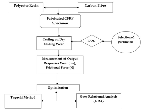
In this work, polyester resin is cured with addition of carbon fibres of size 85 µm in a mild steel mould of dimensions Ø1.5cm ×15cm in height. Figure 1 portrays the research methodology for fabrication and optimization of CFRP composites.
Figure 1. Methodology of current research
2.2 Composite fabrication
Due to addition of hardeners Methyl Ethyl Ketone Peroxide (MEKP) and Cobalt octoate (CO) unsaturated polyester resin is cured with carbon fiber of 85 µm in size. Table 1 depicts the composition of various composites. Before pouring the resin into the mould the releasing agent is applied. For better yield of the casting semi solid state mixture is held for 24 hours at ambient conditions. After 24 hours specimens are withdrawn from the mould and are machined to 8 mm diameter at RVR & JC College of engineering and specimens were polished for wear tests in a calibrated machine.
Table 1. The composition of various composites
|
Sl. no |
Identification of Composite |
Wt% of Carbon fiber |
Wt% of Polyester resin |
Wt% of Hardener (MEKP+CO) |
|
1. |
100% Pure Polyester |
0 |
200 |
2 |
|
2. |
2Wt% CF + 98% Polyester |
2 |
200 |
4 |
|
3. |
4Wt% CF + 96% Polyester |
4 |
200 |
6 |
|
4. |
6Wt% CF + 94% Polyester |
6 |
200 |
8 |
2.3 Dry-sliding wear test
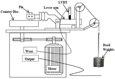
Based on the literature available wear tests were conducted using pin-on-disc tribometer as per ASTM G99-95 standards [17]. Figure 2 depicts the pin on disc tribometer in which wear pins are prepared with dimensions Ø0.8 cm×5 cm in height. The load was imparted on to the pin against its counterpart on an EN32 steel disc during the test. After running over a sliding distance, the pins were removed, gutted with acetone, dried out, and weighted to know the wear due to loss of weight. The loss of wear is determined by difference in weight measured pre and post experimentation. The wear (W in µm) and frictional force (FF in N) of prepared CFRP composites were investigated as a function of normal loads (L), percent of reinforcement (R), sliding velocity (S), and sliding distance (D).
Figure 2. Pin-on-disc tribometer [18]
2.4 Taguchi’s design of experiments (DOE)
Table 2. Control factors and their levels
|
Control Factors |
Levels |
Units |
|||
|
1 |
2 |
3 |
4 |
||
|
S |
2 |
4 |
6 |
8 |
m/s |
|
L |
5 |
10 |
15 |
20 |
N |
|
D |
1000 |
2000 |
3000 |
4000 |
m |
|
R |
0 |
2 |
4 |
6 |
% |
Taguchi experimental design is a versatile method for finding the impacts of multiple parameter effect on response variables. The most critical step in the DOE is picking the monitoring factors that influence the output readings. Initially various factors are taken into account, out of those less significant factors affecting are nullified, leaving only the more significant aspects. In the experimentation of sliding wear, four major factors are taken into account, as shown in Table 2. At room temperature with reference to L16 OA four levels are opted namely load (L), sliding distance (D), sliding velocity (S), and percent of fibre reinforcement (R) and experimentation is conducted. The number of Experiments was decreased from 256 conventional runs to just 16 runs using Taguchi L16 OA, saving both time and money (Table 3). These tests results are converted into signal-to-noise ratios (SNR). To convert S/N ratio logarithmic function is used as shown in Eq. (1) [19-21].
“Smaller-the-Better”,
$S / N_{S B}=-10 \log _{10}\left[\frac{1}{n} \sum_{i=1}^{n} y_{i}^{2}\right]$ (1)
where, n represents number of runs (n=16) and y represents to the output parameters (y=2).
Table 3. L16 OA based on Taguchi approach
|
Runs |
Independent Factors |
|||
|
S |
L |
D |
R |
|
|
1 |
1 |
1 |
1 |
1 |
|
2 |
1 |
2 |
2 |
2 |
|
3 |
1 |
3 |
3 |
3 |
|
4 |
1 |
4 |
4 |
4 |
|
5 |
2 |
1 |
2 |
3 |
|
6 |
2 |
2 |
1 |
4 |
|
7 |
2 |
3 |
4 |
1 |
|
8 |
2 |
4 |
3 |
2 |
|
9 |
3 |
1 |
3 |
4 |
|
10 |
3 |
2 |
4 |
3 |
|
11 |
3 |
3 |
1 |
2 |
|
12 |
3 |
4 |
2 |
1 |
|
13 |
4 |
1 |
4 |
2 |
|
14 |
4 |
2 |
3 |
1 |
|
15 |
4 |
3 |
2 |
4 |
|
16 |
4 |
4 |
1 |
3 |
2.5 Grey Relational analysis (GRA)
To enhance the process parameter in view of single objective Taguchi’s experimental design is enough. When there are two or more responses with different objectives, to optimize them GRA is applied. GRA [22, 23] can also be used to assess the familiarity of unknown data. Due to this reason for multi-objective optimization to evaluate wear parameters GRA approach is used. The ANOVA method identifies important factor that are influencing the wear behaviour. Taguchi GRA combinatorial approach is evaluated using as follows [24, 25]:
Step-I: Wear and frictional force values are normalized based on "Smaller-the-Better" criteria, using Eq. (2).
$y_{i}(k)=\frac{\max x_{i}(k)-x_{i}(k)}{\max x_{i}(k)-\min x_{i}(k)}$ (2)
In Eq. (2), i=1, 2, 3, 4, 5 … 16 (no. of records), k=1, 2 (no. of output parameters), x_i (k) is empirical value, max xi(k) equals to maximum value of xi(k) and min xi(k) equals to minimum value of xi(k).
Step-II: For all process variables using Eq. (3) the deviation sequence determined.
$\Delta_{o i}(k)=\left|x_{o}(k)-x_{i}(k)\right|$ (3)
where, Δoik is the base for both xok & the comparability sequence xik and it is known as deviation sequence.
Step-III: To calculate the GRC (Grey Relational Coefficients) Eq. (3) is used.
$\xi_{i}(k)=\frac{\Delta_{\min }+\zeta \Delta_{\max }}{\Delta_{o i}(k)+\zeta \Delta_{\max }}$ (4)
In Eq. (4), ζ is distinguishing coefficient and its value is calculated in two ways namely equal weights and unequal weights. In equal weight method all the parameters are affecting considered to be equally weighed and its value is 0.5 each. But in real world equal weights are not suggestable and entire scenario changes so the allocation of weights to parameters are done by entropy method.
Step-IV: The main step in employing equation is to anticipate the GRG (Grey Relational Grade) by taking the mean of all GRC values using Eq. (5).
$\gamma_{i}=\frac{1}{n} \sum_{k=1}^{n} \xi_{i}(k)$ (5)
where, γi ranges from 0-1 and ‘n’=number of output readings.
2.6 Entropy method
Shannon Entropy method is used to calculating weights for the various parameters considered i.e., Distinguishing coefficient(ζ). The following method is employed to find the weightage of individual parameters affecting the process.
Step 1: Normalization of the arrays of decision matrix to acquire the project outcomes pij
$p_{i j}=\frac{x_{i j}}{\sum_{i=1}^{m} x_{i j}}$ (6)
Step 2: Computation of the entropy measure of project outcomes using the following equation:
$E_{j}=-K \sum_{i=1}^{m} p_{i j} \log _{e} p_{i j}$ (7)
where, $K=\frac{1}{\log _{e} m}$.
Step 3: Defining the objective weight based on the entropy concept
$w_{j}=\frac{1-E_{j}}{\sum_{j=1}^{n}\left(1-E_{j}\right)}$ (8)
3.1 Implementation of Taguchi method
3.1.1 Calculation of S⁄N ratio
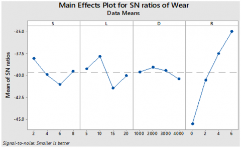
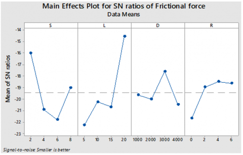
To perform statistical analysis of the experimental records Minitab 19 software was used. Table 4 forecasts wear and frictional force experimental data, as well as the corresponding S/N ratios, whereas Table 5 illustrate S/N ratio responses for wear (W) and frictional force (FF). Figures 3 and 4 depict how the S/N ratio is altered by controlling both the parameters i.e., W & FF. An optimal control factor setting for greater performance can be accomplished by evaluating the lowest S/N ratios values. The lowest S/N ratios are shown in bold in Table 5. Figure 3 and Table 5 illustrate that percent of reinforcement (R) has an impact on wear (W), whereas Figure 4 and Table 5 show that load (L) has an impact on frictional force (FF). Based on S/N ratios, Minitab software throws a combination of parameters to get least wear as shown in Figure 3 and Table 5. Due to amalgamation of parameters least wear is obtained at S1 L2 D2 R4 whereas for minimum frictional force S1 L4 D3 R3 is the optimal condition as in Figure 4 and Table 5.
3.1.2 Analysis of variance
The key control parameters that influence wear and frictional force response values were identified using ANOVA (Analysis of Variance). The significant importance of factors is calculated using the overall sum of squared value. The bigger the total of squared values, the more important it is to manage the response values. These data are used to regulate the percentage contribution on the individual parameters [26]. The study is carried out with a 95% level of confidence and a significance level of 5%. The ANOVA results for wear and frictional force are shown in Tables 6 and 7, respectively. According to Table 6, the most important factor impacting wear is R which contributes for 65.61%, followed by L, S, and D, which contribute for 12.34%, 7.71%, and 5.35%, respectively. According to Table 7, the most important factor dominating frictional force is L which contributes about 43.85%, followed by S which contributes 31.71%, R which contributes 9.18%, and D which contributes almost 9.00%. A high F-value signifies those factors selected as a major influencing on the performance of the process [27, 28].
Figure 3. Main effect of wear for the S⁄N ratio plots
Table 4. Multi-response outputs along with S⁄N ratio for Taguchi L16 OA
|
Runs |
Control Factors |
Response variables |
S⁄N Ratios |
|||||
|
S (m/s) |
L (N) |
D (m) |
R (%) |
W (µm) |
FF (N) |
W (dB) |
FF (dB) |
|
|
1 |
2 |
5 |
1000 |
0 |
162 |
10.5 |
-44.1903 |
-20.4238 |
|
2 |
2 |
10 |
2000 |
2 |
83 |
7.25 |
-38.3816 |
-17.2068 |
|
3 |
2 |
15 |
3000 |
4 |
63 |
5.12 |
-35.9868 |
-14.1854 |
|
4 |
2 |
20 |
4000 |
6 |
48 |
4.11 |
-33.6248 |
-12.2768 |
|
5 |
4 |
5 |
2000 |
4 |
62 |
16.3 |
-35.8478 |
-24.2438 |
|
6 |
4 |
10 |
1000 |
6 |
39 |
11.03 |
-31.8213 |
-20.8515 |
|
7 |
4 |
15 |
4000 |
0 |
325 |
19.25 |
-50.2377 |
-25.6886 |
|
8 |
4 |
20 |
3000 |
2 |
121 |
4.39 |
-41.6557 |
-12.8493 |
|
9 |
6 |
5 |
3000 |
6 |
76 |
12.91 |
-37.6163 |
-22.2185 |
|
10 |
6 |
10 |
4000 |
4 |
84 |
12.36 |
-38.4856 |
-21.8404 |
|
11 |
6 |
15 |
1000 |
2 |
138 |
15.25 |
-42.7976 |
-23.6654 |
|
12 |
6 |
20 |
2000 |
0 |
184 |
9.32 |
-45.2964 |
-19.3883 |
|
13 |
8 |
5 |
4000 |
2 |
92 |
12.76 |
-39.2758 |
-22.1170 |
|
14 |
8 |
10 |
3000 |
0 |
133 |
11.37 |
-42.4770 |
-21.1152 |
|
15 |
8 |
15 |
2000 |
6 |
69 |
9.1 |
-36.7770 |
-19.1808 |
|
16 |
8 |
20 |
1000 |
4 |
95 |
4.83 |
-39.5545 |
-13.6789 |
Table 5. Response table for wear and frictional force based on S⁄N ratio
|
|
Wear |
Frictional force |
||||||
|
Level |
S |
L |
D |
R |
S |
L |
D |
R |
|
1 |
-38.05 |
-39.23 |
-39.59 |
-45.55 |
-16.02 |
-22.25 |
-19.65 |
-21.65 |
|
2 |
-39.89 |
-37.79 |
-39.08 |
-40.53 |
-20.91 |
-20.25 |
-20 |
-18.96 |
|
3 |
-41.05 |
-41.45 |
-39.43 |
-37.47 |
-21.78 |
-20.68 |
-17.59 |
-18.49 |
|
4 |
-39.52 |
-40.03 |
-40.41 |
-34.96 |
-19.02 |
-14.55 |
-20.48 |
-18.63 |
|
Delta |
3 |
3.66 |
1.33 |
10.59 |
5.75 |
7.7 |
2.89 |
3.17 |
|
Rank |
3 |
2 |
4 |
1 |
2 |
1 |
4 |
3 |
Figure 4. Main effect of frictional force for the S⁄N ratio plots
Table 6. ANOVA table for the S⁄N ratio of wear
|
Source |
SS a |
DF b |
MS c |
F-value |
P-value |
Contribution % |
|
S |
5705 |
3 |
1902 |
0.86 |
0.549 |
7.71 |
|
L |
9136 |
3 |
3045 |
1.37 |
0.4 |
12.34 |
|
D |
3960 |
3 |
1320 |
0.6 |
0.66 |
5.35 |
|
R |
48561 |
3 |
16187 |
7.3 |
0.068 |
65.61 |
|
Error |
6653 |
3 |
2218 |
|
|
8.99 |
|
Total |
74016 |
15 |
|
|
|
100.00 |
|
S=47.09, R2=91.01%, R2adj=55.06% |
||||||
Table 7. ANOVA table for the S⁄N ratio of frictional force
|
Source |
SS a |
DF b |
MS c |
F-value |
P-value |
Contribution % |
|
S |
95.47 |
3 |
31.825 |
5.07 |
0.108 |
31.71 |
|
L |
132.01 |
3 |
44.004 |
7.01 |
0.072 |
43.85 |
|
D |
27.1 |
3 |
9.033 |
1.44 |
0.386 |
9.00 |
|
R |
27.65 |
3 |
9.218 |
1.47 |
0.38 |
9.18 |
|
Error |
18.82 |
3 |
6.275 |
|
|
6.25 |
|
Total |
301.06 |
15 |
|
|
|
100.00 |
|
S=2.50, R2=93.75%, R2adj=68.74% |
||||||
|
a Sum of Squares. b Degrees of Freedom. c Mean squares. |
||||||
Table 6 depicts that % reinforcement is the major contributing factor change in wear. Similarly, in Table 7 load is the major factor affecting change in frictional force. From Table 6 and 7 based on the R2 (i.e., coefficient of correlation) one may predict that the model as good linear fit with less error [29, 30].
3.2 Multi-response optimization using GRA
Wear and frictional force are two characteristics that occur simultaneously. Consequently, they need to be optimized in tandem. GRA was chosen for this purpose since it has the ability to reduce a multi-objective problem to a single-objective problem from which it can be optimized [31].
3.2.1 Calculation of GRG
Using Eq. (3) based on the normalized values, deviation sequences are evaluated followed by calculations of GRC and GRG for all responses. The bold values in Table 8 signify that experimental run (4) has the maximum GRG value of 1.00, thereby indicating it as the optimal value. Using Eq. (3) based on the normalized values, deviation sequences are evaluated followed by calculations of GRC and GRG for all responses. The bold values in Table 8 signify that experimental run (4) has the maximum GRG value of 1.00, thereby indicating it as the optimal value. Using the equations i.e., from Eq. (6) to Eq. (8) the entropy weights of wear and frictional force are found to be 0.217, 0.783 and based on that GRG score is evaluated and mentioned in Table 9.
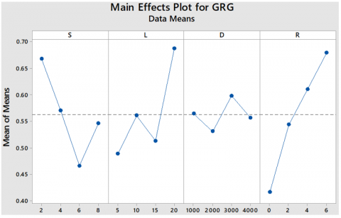
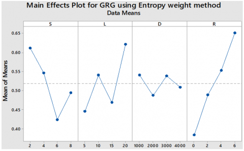
For each parameter based on EWM and EBW methods, GRG responses are evaluated and are depicted in Table 10. Figure 5 and Figure 6 illustrates the main effect plots of GRG using Equal weighted method and Entropy based weight method. Based on EWM method S1 L4 D3 R4 is the optimised condition whereas for EBWM method S1 L4 D1 R4 is the optimal value obtained. The higher the GRG, the closer the product's quality is to its ideal value. As a result, a greater GRG is required for optimal performance.
Figure 5. Main effect plots of GRG using EWM
Figure 6. Main effect plots of GRG using EBWM
Table 8. Calculation of GRC and GRG for wear and frictional force based on equal weightage method (EWM)
|
Runs |
Normalized data [yi(k)] |
Deviation sequence [Δoi(k)] |
GRC [ξi(k)] |
GRG (γi) |
Rank |
|||
|
W |
FF |
W |
FF |
W |
FF |
|||
|
1 |
0.328 |
0.393 |
0.672 |
0.607 |
0.427 |
0.451 |
0.439 |
14 |
|
2 |
0.644 |
0.632 |
0.356 |
0.368 |
0.584 |
0.576 |
0.580 |
6 |
|
3 |
0.774 |
0.858 |
0.226 |
0.142 |
0.689 |
0.778 |
0.733 |
2 |
|
4 |
0.902 |
1.000 |
0.098 |
0.000 |
0.836 |
1.000 |
0.918 |
1 |
|
5 |
0.781 |
0.108 |
0.219 |
0.892 |
0.696 |
0.359 |
0.527 |
8 |
|
6 |
1.000 |
0.361 |
0.000 |
0.639 |
1.000 |
0.439 |
0.719 |
3 |
|
7 |
0.000 |
0.000 |
1.000 |
1.000 |
0.333 |
0.333 |
0.333 |
16 |
|
8 |
0.466 |
0.957 |
0.534 |
0.043 |
0.484 |
0.921 |
0.702 |
4 |
|
9 |
0.685 |
0.259 |
0.315 |
0.741 |
0.614 |
0.403 |
0.508 |
9 |
|
10 |
0.638 |
0.287 |
0.362 |
0.713 |
0.580 |
0.412 |
0.496 |
10 |
|
11 |
0.404 |
0.151 |
0.596 |
0.849 |
0.456 |
0.371 |
0.413 |
15 |
|
12 |
0.268 |
0.470 |
0.732 |
0.530 |
0.406 |
0.485 |
0.446 |
13 |
|
13 |
0.595 |
0.266 |
0.405 |
0.734 |
0.553 |
0.405 |
0.479 |
11 |
|
14 |
0.421 |
0.341 |
0.579 |
0.659 |
0.464 |
0.431 |
0.447 |
12 |
|
15 |
0.731 |
0.485 |
0.269 |
0.515 |
0.650 |
0.493 |
0.571 |
7 |
|
16 |
0.580 |
0.895 |
0.420 |
0.105 |
0.544 |
0.827 |
0.685 |
5 |
Table 9. Calculation of GRC and GRG for wear and frictional force based on entropy based weightage method (EBWM)
|
Runs |
Normalized data [yi(k)] |
Deviation sequence [Δoi(k)] |
GRC [ξi(k)] |
GRG (γi) |
Rank |
|||
|
W |
FF |
W |
FF |
W |
FF |
|||
|
1 |
0.328 |
0.393 |
0.672 |
0.607 |
0.245 |
0.563 |
0.404 |
14 |
|
2 |
0.644 |
0.632 |
0.356 |
0.368 |
0.379 |
0.680 |
0.530 |
6 |
|
3 |
0.774 |
0.858 |
0.226 |
0.142 |
0.490 |
0.846 |
0.668 |
3 |
|
4 |
0.902 |
1.000 |
0.098 |
0.000 |
0.689 |
1.000 |
0.845 |
1 |
|
5 |
0.781 |
0.108 |
0.219 |
0.892 |
0.499 |
0.467 |
0.483 |
8 |
|
6 |
1.000 |
0.361 |
0.000 |
0.639 |
1.000 |
0.550 |
0.775 |
2 |
|
7 |
0.000 |
0.000 |
1.000 |
1.000 |
0.179 |
0.439 |
0.309 |
16 |
|
8 |
0.466 |
0.957 |
0.534 |
0.043 |
0.289 |
0.948 |
0.619 |
4 |
|
9 |
0.685 |
0.259 |
0.315 |
0.741 |
0.409 |
0.514 |
0.461 |
9 |
|
10. |
0.638 |
0.287 |
0.362 |
0.713 |
0.375 |
0.523 |
0.449 |
10 |
|
11. |
0.404 |
0.151 |
0.596 |
0.849 |
0.267 |
0.480 |
0.373 |
15 |
|
12. |
0.268 |
0.470 |
0.732 |
0.530 |
0.229 |
0.596 |
0.413 |
12 |
|
13 |
0.595 |
0.266 |
0.405 |
0.734 |
0.349 |
0.516 |
0.433 |
11 |
|
14 |
0.421 |
0.341 |
0.579 |
0.659 |
0.273 |
0.543 |
0.408 |
13 |
|
15 |
0.731 |
0.485 |
0.269 |
0.515 |
0.447 |
0.603 |
0.525 |
7 |
|
16 |
0.580 |
0.895 |
0.420 |
0.105 |
0.341 |
0.882 |
0.612 |
5 |
Table 10. GRG response table using EWM and EBWM
|
|
Equal weightage method (EWM) |
Entropy based weightage method (EBWM) |
||||||
|
Level |
S |
L |
D |
R |
S |
L |
D |
R |
|
1 |
0.6677 |
0.4885 |
0.5643 |
0.4164 |
0.6116 |
0.4451 |
0.541 |
0.3833 |
|
2 |
0.5707 |
0.5608 |
0.5312 |
0.5437 |
0.5464 |
0.5405 |
0.4876 |
0.4887 |
|
3 |
0.4659 |
0.5129 |
0.5979 |
0.6106 |
0.4241 |
0.4688 |
0.539 |
0.553 |
|
4 |
0.5458 |
0.6879 |
0.5566 |
0.6793 |
0.4944 |
0.6219 |
0.5089 |
0.6515 |
|
Delta |
0.2018 |
0.1994 |
0.0668 |
0.2629 |
0.1875 |
0.1768 |
0.0534 |
0.2682 |
|
Rank |
2 |
3 |
4 |
1 |
2 |
3 |
4 |
1 |
Table 11. ANOVA table for GRG using EWM
|
Source |
SS a |
DOF b |
MS c |
F-value |
P-value |
Contribution % |
|
S |
0.083014 |
3 |
0.027671 |
7.99 |
0.061 |
23.87 |
|
L |
0.094656 |
3 |
0.031552 |
9.11 |
0.051 |
27.22 |
|
D |
0.0091 |
3 |
0.003033 |
0.88 |
0.542 |
2.62 |
|
R |
0.150627 |
3 |
0.050209 |
14.5 |
0.027 |
43.31 |
|
Error |
0.010386 |
3 |
0.003462 |
|
|
2.99 |
|
Total |
0.347783 |
15 |
|
|
|
100.00 |
|
S=0.0588, R2=97.01%, R2adj=85.07% |
||||||
Table 12. ANOVA table for GRG using EBWM
|
Source |
SS a |
DOF b |
MS c |
F-value |
P-value |
Contribution % |
|
S |
0.075747 |
3 |
0.025249 |
3.8 |
0.151 |
22.82 |
|
L |
0.076122 |
3 |
0.025374 |
3.82 |
0.15 |
22.94 |
|
D |
0.007899 |
3 |
0.002633 |
0.4 |
0.766 |
2.38 |
|
R |
0.152201 |
3 |
0.050734 |
7.64 |
0.065 |
45.86 |
|
Error |
0.019934 |
3 |
0.006645 |
|
|
6.01 |
|
Total |
0.331903 |
15 |
|
|
100.00 |
|
|
S=0.0815, R2=93.99%, R2adj=69.97% |
||||||
|
a Sum of Squares. b Degrees of Freedom (DOF) c Mean squares. |
||||||
3.2.2 ANOVA for GRG
Analysis of Variance (ANOVA) is used to examine aspects which have a substantial influence on an individual's performance. This is performed by dividing total GRG variability, as measured by the sum of squared deviations from the GRG's average value into contributions from each wear parameter and listing them in Table 11 and 12. For each parameter based on EWM and EBWM methods, ANNOVA analysis is performed are evaluated. The ANOVA results for EWM and EBWM methods are shown in Tables 11 and 12, respectively. According to Table 11, the most important factor affecting EWM method is R which contributes for 43.31%, followed by L, S, and D, which contribute for 27.22%, 23.87%, and 2.62%, respectively whereas Table 12 depicts the contributions of factors affecting under the influence of unequal weights (EBW method). The most important factor affecting EBWM method is R which contributes for 45.86%, followed by L, S, and D, which contribute for 22.94%, 22.82%, and 2.38%.
3.2.3 Confirmation test
A confirmation test was done to validate experimental results based on the discovery of the ideal parameter's effecting numerous replies. The projected GRG is calculated using Eq. (9). Table 13 shows that the expected and experimental results are nearly identical for both the EWM and EBW method. Thus, indicating that the study was carried out satisfactorily. The measured GRG for the optimal combo level in EWM is 0.868, while the expected GRG is 0.869 whereas for EBW method experimental value is 0.943 while the expected GRG is 0.945. The experimental and expected outcomes were very similar. As a result, the grey relation approach is useful for optimising the wear parameter when numerous attributes must be investigated at the same time [32].
$\hat{y}=y_{m}+\sum_{i=1}^{q}\left(\bar{y}_{\imath}-y_{m}\right)$ (9)
where, $\hat{y}$ means predicted grey relation grade, ym means average value of GRG, yi GRG at optimum levels and q equals to number of factors.
Table 13. Confirmation test readings
|
|
Best process parameters |
|
|
Expected |
Investigational |
|
|
Using Entropy weight method |
S1 L4 D1 R4 |
S1 L4 D1 R4 |
|
GRG |
0.869 |
0.868 |
|
Equal weights consideration |
S1 L4 D3 R4 |
S1 L4 D3 R4 |
|
GRG |
0.945 |
0.943 |
Both the methods have been successively applied to forecast the of wear behaviour of Polyester composite using GRA technique. The best experimental conditions have been considered and closely matched to predicted values within the margin of minimum error. EWM method calculates the GRC by considering all variables with equal importance however EBW method decides the weightages depending upon variation in larger to smaller values. Even though both methods produced satisfactory results it is up to the decision maker to choose the weightage scenario depending upon the condition and application.
Die casting technique was used to create polyester composites with carbon fiber additions rising from 2 to 6 Wt% at 2 Wt% intervals. The findings show that increasing the content of carbon fibers reduces the sliding wear dramatically.
[1] Velmurugan, K., Gopinath, R. (2015). Characterization of polyester based composites. International Journal of Science, 4(7).
[2] Bagherpour, S. (2012). Fibre Reinforced Polyester Composites. London: InTech. pp. 135-166.
[3] Black, T., Kosher, R. (2008). Non metallic materials: Plastic, elastomers, ceramics and composites. Materials and Processing in Manufacturing, 10: 162-194.
[4] Pıhtılı, H., Tosun, N. (2002). Investigation of the wear behaviour of a glass-fibre-reinforced composite and plain polyester resin. Composites Science and Technology, 62(3): 367-370. https://doi.org/10.1016/s0266-3538(01)00196-8
[5] Hutchings, I.M. (1994). Wear-resistant materials: Into the next century. Materials Science and Engineering: A, 184(2): 185-195. https://doi.org/10.1016/0921-5093(94)91031-6
[6] Ahmed, I.R., Yousry, A.W. (2012). Tribological properties of polyester composites: Effects of vegetable oils and polymer fibers. Polyester, 203-226. https://doi.org/10.5772/39230
[7] Messana, A., Sisca, L., Ferraris, A., Airale, A.G., de Carvalho Pinheiro, H., Sanfilippo, P., Carello, M. (2019). From design to manufacture of a carbon fiber monocoque for a three-wheeler vehicle prototype. Materials, 12(3): 332. https://doi.org/10.3390/ma12030332
[8] Soutis, C. (2005). Fibre reinforced composites in aircraft construction. Progress in Aerospace Sciences, 41(2): 143-151. https://doi.org/10.1016/j.paerosci.2005.02.004
[9] Niedermann, P., Szebényi, G., Toldy, A. (2015). Characterization of high glass transition temperature sugar-based epoxy resin composites with jute and carbon fibre reinforcement. Composites Science and Technology, 117: 62-68. http://dx.doi.org/10.1016/j.compscitech.2015.06.001
[10] Davim, J.P., Marques, N., Baptista, A.M. (2001). Effect of carbon fibre reinforcement in the frictional behaviour of Peek in a water lubricated environment. Wear, 251(1-12): 1100-1104. https://doi.org/10.1016/S0043-1648(01)00741-4
[11] Kumar, S., Sai Ram, Y.N.V. (2022). Tribological behaviour of carbon fiber reinforced polyester composites. In: Kumari R., Majumdar J.D., Behera A. (eds) Recent Advances in Manufacturing Processes. Lecture Notes in Mechanical Engineering. Springer, Singapore. https://doi.org/10.1007/978-981-16-3686-8_1
[12] Tzeng, G.H., Huang, J.J. (2011). Multiple Attribute Decision Making: Methods and Applications. CRC Press. https://doi.org/10.1201/b11032
[13] Sreenivasulu, R. (2013). Optimization of surface roughness and delamination damage of GFRP composite material in end milling using Taguchi design method and artificial neural network. Procedia Engineering, 64: 785-794. https://doi.org/10.1016/j.proeng.2013.09.154
[14] Rao, D.K., Srinivas, K. (2017). An analysis of feature identification for tool wear monitoring by using acoustic emission. Traitement du Signal, 34(3-4): 117. https://doi.org/10.3166/ts.34.117-135
[15] Sreenivasulu, R., Rao, C.S. (2016). Effect of drilling parameters on thrust force and torque during drilling of aluminium 6061 alloy-based on Taguchi design of experiments. Journal of Mechanical Engineering, 46(1): 41-48. https://doi.org/10.3329/jme.v46i1.32522
[16] Geeth, K.M., Reddy, M.C.S., Kumar, M.S. (2021). Optimization of dry-sliding wear parameters on carbon fiber reinforced polyester composites using Taguchi based Greyrelation analysis. In IOP Conference Series: Materials Science and Engineering, 1185(1): 012003. https://doi.org/10.1088/1757-899x/1185/1/012003
[17] Ram, Y.S., Kammaluddin, S., Raj, C.D., MastanRao, P. (2016). Sliding wear behavior of high velocity oxy-fuel sprayed WC-CO coatings. International Journal of Advanced Science and Technology, 93: 45-54. http://dx.doi.org/10.14257/ijast.2016.93.05
[18] Mohapatra, S.K., Maity, K. (2017). Synthesis and characterisation of hot extruded aluminium-based MMC developed by powder metallurgy route. International Journal of Mechanical and Materials Engineering, 12(1): 1-9. http://dx.doi.org/10.1186/s40712-016-0068-9
[19] Cherukuri, T., Kommineni, R. (2017). Application of taguchi techniques to study dry sliding wear behaviour of magnesium matrix composites reinforced with alumina nano particles. Journal of Engineering Science and Technology, 12: 2855-2865.
[20] TR, H.K., Swamy, R.P., Chandrashekar, T.K. (2011). Taguchi technique for the simultaneous optimization of tribological parameters in metal matrix composite. Journal of Minerals & Materials Characterization & Engineering, 10(12): 1179-1188. http://dx.doi.org/10.4236/jmmce.2011.1012090
[21] Kalita, K., Ghadai, R.K., Bansod, A. (2022). Sensitivity analysis of GFRP composite drilling parameters and genetic algorithm-based optimisation. International Journal of Applied Metaheuristic Computing (IJAMC), 13(1): 1-17. https://doi.org/10.4018/IJAMC.290539
[22] Achuthamenon, S.P., Ramakrishnasamy, R., Palaniappan, G. (2018). Taguchi grey relational analysis for multi-response optimization of wear in co-continuous composite. Materials, 11(9): 1743 https://doi.org/10.3390/ma11091743
[23] Antil, P., Singh, S., Manna, A. (2018). Electrochemical discharge drilling of SiC reinforced polymer matrix composite using Taguchi’s grey relational analysis. Arabian Journal for Science and Engineering, 43(3): 1257-1266. https://doi.org/10.1007/513369-017-2882-6
[24] Tarasasanka, C., Snehita, K., Ravindra, K., Sameerkumar, D. (2019). Optimization of dry sliding wear properties of AZ91E/nano Al2O3 reinforced metal matrix composite with grey relational analysis. International Journal of Engineering, Science and Technology, 11(4): 41-48. http://dx.doi.org/10.4314/ijest.v11i4.4
[25] Raju, S.S., Senapathi, A.K., Rao, G.S. (2017). Estimation of tribological performance of Al-MMC reinforced with a novel in-situ ternary mixture using grey relational analysis. Indian Journal of Science and Technology, 10(15): 1-9. http://dx.doi.org/10.17485/ijst/2017/v10i15/113825
[26] Çiçek, A., Kıvak, T., Ekici, E. (2015). Optimization of drilling parameters using Taguchi technique and response surface methodology (RSM) in drilling of AISI 304 steel with cryogenically treated HSS drills. Journal of Intelligent Manufacturing, 26(2): 295-305. http://dx.doi.org/10.1007/s10845-013-0783-5
[27] Sudheer, M., Prabhu, R., Raju, K., Bhat, T. (2013). Modeling and analysis for wear performance in dry sliding of Epoxy/Glass/PTW composites using full factorial techniques. International Scholarly Research Notices, 2013. https://doi.org/10.5402/2013/624813
[28] Kilickap, E., Yardimeden, A., Çelik, Y.H. (2017). Mathematical modelling and optimization of cutting force, tool wear and surface roughness by using artificial neural network and response surface methodology in milling of Ti-6242S. Applied Sciences, 7(10): 1064. https://doi.org/10.3390/app7101064
[29] Rakić, T., Kasagić-Vujanović, I., Jovanović, M., Jančić-Stojanović, B., Ivanović, D. (2014). Comparison of full factorial design, central composite design, and box-Behnken design in chromatographic method development for the determination of fluconazole and its impurities. Analytical Letters, 47(8): 1334-1347. https://doi.org/10.1080/00032719.2013.867503
[30] Wojciechowski, S., Maruda, R.W., Krolczyk, G.M., Niesłony, P. (2018). Application of signal to noise ratio and grey relational analysis to minimize forces and vibrations during precise ball end milling. Precision Engineering, 51: 582-596. https://doi.org/10.1016/j.precisioneng.2017.10.014
[31] Siriyala, R., Alluru, G.K., Penmetsa, R.M.R., Duraiselvam, M. (2012). Application of Grey-Taguchi method for optimization of dry sliding wear properties of aluminum MMCs. Frontiers of Mechanical Engineering, 7(3): 279-287. https://doi.org/10.1007/s11465-012-0329-0
[32] Laxminarayana, P. (2018). Optimization of electrode tool wear in micro holes machining by die sinker EDM using Taguchi approach. Materials Today: Proceedings, 5(1): 1824-1831. https://doi.org/10.1016/j.matpr.2017.11.281