Delin Sun* | Lingling Zhao | Guihang Liang | Huawei Zhou
OPEN ACCESS
In factory-assembled structures, the bolted joint is the cause of local energy dissipation and flexibility, and its dynamics influences the dynamics of the whole structure. This paper puts forward a method to simulate the dynamics of bolted joint based on the thin-layer element (TLE) of nonlinear material. First, a finite-element model was built for an isolated bolted joint. Then, the tangential force-displacement curve of the bolted joint was obtained through an experiment on a universal testing machine (UTM) to reflect the features of the joint. On this basis, the response surface methodology (RSM) and the genetic algorithm (GA) were combined to identify the parameters of the material in the finite-element model. The simulated force-displacement curve agrees well with that measured through experiment. Our approach facilitates the precise prediction of the dynamics of factory-assembled structures with complex joints.
bolted joint, thin-layer element (TLE), stiffness, finite-element model
Bolted joints are one of the most common elements in factory-assembled structures. Traditionally, the dynamics of a factory-assembled structure is simulated by a finite-element model, and the stiffness of the structure is expressed by a rigid joint or spring, without considering the damping features. The modal frequency, shape and damping are determined through experiments.
Through parameter adjustment, the linear structural model provides an efficient way to approximate the modal frequency and damping, and compute the structural response if the conditions are similar to experimental ones [1-6]. However, there are two major problems with this approach. First, the linear structural model cannot make a prediction without a physical prototype. Second, the simulated dynamic strength will deviate greatly from the measured value, if the actual load is far beyond the simulated load, due to the highly nonlinear damping and stiffness of the joint.
The key to predicting the dynamics of the factory-assembled structure lies in the constitutive modelling of the joint [7-9]. An effective constitutive model must carry the following features: the model should be able to reproduce the main features of the joint response; the model parameters should be derived systematically from the test data or finite-element modeling results of the joint; the model should be easy to integrate into finite-element software.
The classical solution is to simulate the damping and stiffness features of the joint by parameterized Iwan model [10, 11]. This solution involves three steps: establish the parameterized Iwan model, identify the model parameters based on the data of isolated joint test, and embed the model into the finite-element model. However, the Iwan model has not been effectively transplanted to the existing commercial software.
In view of the above, this paper proposes a new method to simulate the dynamic features of bolted joint based on the thin-layer element (TLE) of nonlinear material. First, the TLE method and the constitutive structure of shear stiffness were introduced. Then, a parameterized Richard-Abbot material model was set up using the function of user-defined material of Abaqus. Next, a finite-element model was established for isolated bolted joint. After that, the tangential force-displacement curve reflecting the features of the bolted joint were acquired through experiments on a universal testing machine (UTM). Finally, the material parameters of the TLE were identified.
2.1 The TLE method
The TLE method is an approach to model the joint surface. It was initially developed to model the rock interface, which features thin elements and a large width-to-thickness ratio. The constitutive model of the thin elements can be expressed as the matrix below:
$\left\{ \begin{matrix} {{\sigma }_{1}} \\ {{\sigma }_{2}} \\ {{\sigma }_{3}} \\ {{\tau }_{12}} \\ {{\tau }_{23}} \\ {{\tau }_{31}} \\\end{matrix} \right\}=\left[ \begin{matrix} {{c}_{11}} & {{c}_{12}} & {{c}_{13}} & {{c}_{14}} & {{c}_{15}} & {{c}_{16}} \\ {} & {{c}_{22}} & {{c}_{23}} & {{c}_{24}} & {{c}_{25}} & {{c}_{26}} \\ {} & {} & {{c}_{33}} & {{c}_{34}} & {{c}_{35}} & {{c}_{36}} \\ {} & {} & {} & {{c}_{44}} & {{c}_{45}} & {{c}_{46}} \\ {} & {} & {} & {} & {{c}_{55}} & {{c}_{56}} \\ Sym. & {} & {} & {} & {} & {{c}_{66}} \\\end{matrix} \right]\left\{ \begin{matrix} {{\varepsilon }_{1}} \\ {{\varepsilon }_{2}} \\ {{\varepsilon }_{3}} \\ {{\gamma }_{12}} \\ {{\gamma }_{23}} \\ {{\gamma }_{31}} \\\end{matrix} \right\}$ (1)
where, cij are unknown parameters. The number of unknown parameters can be reduced based on reasonable physical assumptions. Mayer and Gaul put forward four assumptions for these parameters: (1) The nondiagonal elements are zeros, because the joint surface does not shrink in the transverse direction.
(2) The parameters c11 and c22 are negligible, due to the lack of stiffness along the interface parallel to the joint surface.
(3) The normal stiffness of the joint is reflected by c33, while the shear stiffness of the joint is defined by c55=c66.
(4) The parameter c44 is zero, due to the absence of in-plane shear stiffness.
According to the above assumptions, the constitutive model only contains the physical quantities that are perpendicular to the normal direction and parallel to the tangential direction of the joint surface.
2.2 Constitutive relation of shear stiffness
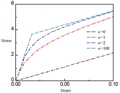
For a jointed structure, the increase in the excitation amplitude will push up the nonlinearity of the mechanical joint, which brings about two phenomena: the weakening stiffness and growing friction damping. To characterize the two phenomena, a nonlinear Richard-Abbot model was introduced to describe the stress-strain relationship in the tangential direction of the elements on the joint surface [12-14]:
$\sigma=\frac{\left(E_{e}-E_{p}\right) \varepsilon}{\left(1+\left|\frac{\left(E_{e}-E_{p}\right) \varepsilon}{S_{Y}}\right|^{n}\right)^{1 / n}}+E_{p} \varepsilon$ (2)
where, Ee and Ep are stick elastic stiffness and slip plastic stiffness, respectively; Sy is the yield point; n is the shape factor that controls the smoothness of the transition portion of the curve.
Figure 1. Stress-strain curves of different shape factors
Figure 1 shows the stress-strain curves of different shape factors. It can be seen that, when n=0, the curve takes the traditional linear form; with the increase of the shape factor, the stress-strain curve gradually approaches the smooth nonlinear form, which is suitable to describe the transition from stick state to micro-slip state or macro-slip state; as the shape factor further increases (n→∞), the curve approximates the bilinear elastoplastic shape (n=100). Therefore, the nonlinear Richard-Abbot model can describe the load-displacement backbone curves about the stick and micro-slip on the surface of a mechanical joint under external loads. With four unknown parameters (Ee , Ep, Sy and n), this parameterized constitutive model can be integrated into the main program of Abaqus, using the user-defined material function (VUMAT).
3.1 Finite-element modelling and load-displacement calculation
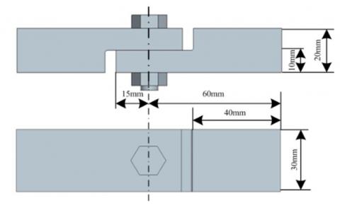
As shown in Figure 2, the bolted joint in our research consists of two metal plates, one bolt and one nut (M8). The material properties of the bolt components are listed in Table 1.
Figure 2. Bolted joint
Table 1. Material properties of the bolted joint
|
Component |
Material |
Young’s modulus/GPa |
Poisson’s ratio |
|
Metal plates |
2Cr13 |
2.06 |
0.3 |
|
Bolt and nut |
06Cr19Ni10 |
1.94 |
0.3 |
3.2 Finite-element model and boundary conditions
Figure 3 presents the finite-element model of the bolted joint based on hexahedron grids. To impose the displacement and output the reaction forces, a reference point was established and connected with the right end of the joint. It can be seen from Figure 3 that the left end of the joint is fixed, while the right end retains tangential freedom only.
Figure 3. Finite-element model and boundary conditions
3.3 Numerical results
Table 2 provides the initial values of the model parameters. Suppose the reference point is subjected to a displacement load of 0.01mm. The model can be solved to obtain the corresponding reaction forces [15].
Table 2. Initial values of model parameters
|
Parameter |
Symbol |
Value |
|
Normal elastic stiffness |
En |
2,000MPa |
|
Stick elastic stiffness |
Ee |
220MPa |
|
Slip plastic stiffness |
Ep |
22MPa |
|
Yield point |
Sy |
5.3MPa |
|
Shape factor |
n |
1.8 |
Then pairs of load-displacement data were extracted at equal intervals. The numerical results on the initial load-displacement curve are shown in Figure 6.
3.4 Experimental measurement
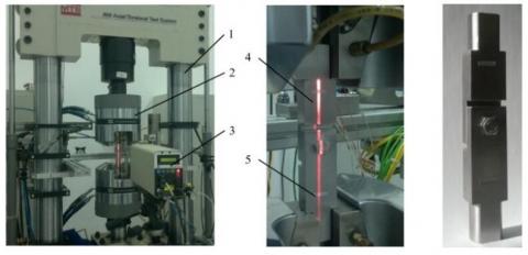
Our tensile experiment was carried out on a self-made lap joint, a type of bolted joint, using a UTM (MTS Criterion). As shown in Figure 4, the UTM contains an MTS 647 wedge-shaped hydraulic gripper, which keeps the bolted joint tightly at both ends throughout the experiment. The gripper has an embedded force sensor (resolution: 1N), which measures the load on the joint. During the experiment, the displacement of the joint was measured by a LX 500 laser extensometer (MTS Criterion). The displacement could be measured to the accuracy of 1μm, by detecting the position marked by a reflective strip. The UTM is connected to a computer workstation, which has the professional software for load control and data recording [16].
Figure 4. The experimental devices (1. UTM; 2. Hydraulic gripper; 3. Laser extensometer; 4. Lap joint; 5. Reflective strip)
3.5 Loading conditions and results
First, the cylinder of the metal plates was inserted into the gripper, properly aligned and fixed. Then, the bolt and the nut were installed, and applied a tightening torque of 20 Nm with a digital torque spanner. Next, a tangential load was applied to the lap joint under the displacement control mode. The displacement was limited to 0.010 mm. The load and displacement values were recorded synchronously. The load-displacement curves obtained through experimental measurement and numerical calculation are both displayed in Figure 6.
The model parameters in Table 2 are essentially function of the preload, roughness and material of the joint surface. These functions determine the stick and micro-slip of the joint surface. The parameters of the TLM in the finite-element model can be corrected effectively by minimizing the difference between the numerical and experimental load-displacement curves. The tangential load Finum obtained by numerical calculation can be described as:
$F_{i}^{\mathrm{num}}=f\left(x_{i}, E_{n}, E_{e}, E_{p}, S_{Y}, n\right)$ (3)
where, xi are the discrete displacements. Then, the objective function can be optimized as:
Objective function$=\sum_{i=1}^{10}\left(F_{i}^{\operatorname{num}}-F_{i}^{\mathrm{exp}}\right)^{2}$ (4)
where, Fiexp is the tangential load at displacement xi. In addition to the origin, there are 10 pairs of load-displacement values. Considering its nonlinear material features, the finite-element model is time-consuming and costly to solve directly by an optimization algorithm. Here, the response surface methodology (RSM) and genetic algorithm (GA) are integrated to complete the parameter identification.
4.1 RSM and GA
The RSM is a statistical modelling tool that obtains the relationship between several explanatory variables and one or more response variable through regression analysis. Since its birth in 1951, the RSM has been widely applied in engineering [17-20]. Its creators, Box and Wilson, suggested approximating the relationship by a quadratic polynomial function:
$R \simeq a_{0}+\sum_{i=1}^{N} b_{i} v_{i}+\sum_{i=1}^{N} c_{i i} v_{i}^{2}+\sum_{i j(i<j)} c_{i j} v_{i} v_{j}$ (5)
where, R is the response, i.e. the load Finum; N is the number of input parameters; vi is the encoded values of En, Ee, Ep, SY and n; a, b and c are regression coefficients.
The main idea of the RSM is to approximate the response model of the design of experiments (DOE) through a seires of experiments. Here, the DOE adopts the optimized Latin hypercube design [12, 13].
In the optimization process, the GA was employed to obtain the required parameters. Mimicking the natural selection process, the GA is detailed in the works of Mohan et al. [21-20].
In this paper, the RSM and the GA are integrated in the global leading optimization software, Isight.
4.2 Parameter identification based on Abaqus and Isight
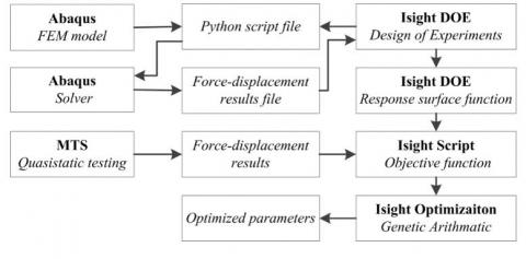
As shown in Figure 5, Abaqus and Isight were combined to establish the response surface function and optimize model parameters. First, the finite-element model of the bolted joint was set up on Abaqus, together with a script file of Python. Being the input for Abaqus solver, the script file contains the entire finite-element model, the boundary and loading conditions, as well as the meshing and model parameters. Through the solving process, the load-displacement relationship was outputted to a destination file. The Python script and Abaqus solver were driven by Isight DOE components to automatically perform the numerical experiments. Table 3 shows the design intervals for the parameters at the time of the DOE. The optimized Latin hypercube technique was used to select 100 sampling points.
Figure 5. The integrated process of parameter identification
Table 3. Design intervals for parameters
|
Parameter |
Symbol |
Lower limit |
Upper limit |
|
Normal elastic stiffness |
En |
1,000 |
10,000 |
|
Stick elastic stiffness |
Ee |
220 |
100 |
|
Slip plastic stiffness |
Ep |
2.2 |
22 |
|
Yield point |
Sy |
1 |
10 |
|
Shape factor |
n |
0.2 |
2 |
The response surface function was defined with the linear least squares (LS) method. The objective function was created with Isight script components, and minimized with the GA. The resulting updated parameters are shown in Table 4.
Table 4. Updated parameters
|
Parameter |
Symbol |
Value |
|
Normal elastic stiffness |
En |
4,260 |
|
Stick elastic stiffness |
Ee |
172 |
|
Slip plastic stiffness |
Ep |
8 |
|
Yield point |
Sy |
3.3 |
|
Shape factor |
n |
0.8 |
Figure 6. Comparison between load-displacement curves obtained through numerical simulation and experiment
As shown in Figure 6, the load-displacement curve obtained through numerical calculation based on the updated parameters only differed slightly from that obtained by the experiment. In other words, the identified data can accurately reflect the response of the isolated bolted joint under external loads.
This paper sets up the finite-element model of a bolted joint, and simulated the joint surface as the TLM of nonlinear material. Then, the tangential force-displacement curve of the bolted joint was obtained through an experiment to reflect the features of the joint. On this basis, the RSM and the GA were combined to identify the parameters of the material in the finite-element model. The identified parameters can accurately characterize the stick-slip response of the material, laying a good basis for computing the dynamic response of factory-assembled structures.
[1] Sone, S.P., Abu, A.B., Nyein, O.K. (2018). Parametric study on vibration response for automobile crankshaft. Asia Proceedings of Social Sciences, 1(4): 85-88. https://doi.org/10.31580/apss.v1i4.460
[2] Adhikari, S. (2006). Damping modelling using generalized proportional damping. Journal of Sound and Vibration, 293(1-2): 156-170. http://dx.doi.org/10.1016/j.jsv.2005.09.034
[3] Sterling, A., Lin, M.C. (2016). Interactive modal sound synthesis using generalized proportional damping. In Proceedings of the 20th ACM SIGGRAPH Symposium on Interactive 3D Graphics and Games, pp. 79-86. http://dx.doi.org/10.1145/2856400.2856419
[4] Zheng, J.L., Peng, M.J., Sun, Y. (2017). Out-plane compressive properties for isosceles trapezoid honeycomb core of FRP Sandwich panel. Journal of Materials Engineering, 45(2): 72-79. https://doi.org/10.11868/j.issn.1001-4381.2014.001534
[5] Abbasloo, A., Maheri, M.R. (2017). Prediction of modal damping of FRP-honeycomb sandwich panels with arbitrary geometries. Latin American Journal of Solids and Structures, 14(1): 17-35. http://dx.doi.org/10.1590/1679-78252537
[6] de Paula Macanhan, V.B., Correa, E.O., de Lima, A.M.G., da Silva, J.T. (2019). Vibration response analysis on stainless steel thin plate weldments. The International Journal of Advanced Manufacturing Technology, 102(5-8): 1779-1786. https://doi.org/10.1007/s00170-019-03297-x
[7] Sun, D., Zhu, M. (2019). Effect of pressure distribution on the energy dissipation of lap joints under equal pre-tension force. Open Physics, 17(1): 320-328. https://doi.org/10.1515/phys-2019-0034
[8] Lee, J., Song, Y., Shin, C.S. (2018). Effect of the sagittal ankle angle at initial contact on energy dissipation in the lower extremity joints during a single-leg landing. Gait & Posture, 62: 99-104. http://dx.doi.org/10.1016/j.gaitpost.2018.03.019
[9] Mayer, M.H., Gaul, L. (2007). Segment-to-segment contact elements for modelling joint interfaces in finite element analysis. Mechanical systems and signal processing, 21(2): 724-734. https://doi.org/10.1016/j.ymssp.2005.10.006
[10] Brake, M.R.W. (2017). A reduced Iwan model that includes pinning for bolted joint mechanics. Nonlinear Dynamics, 87(2): 1335-1349. https://doi.org/10.1007/978-3-319-29763-7_22
[11] Roettgen, D., Allen, M.S., Kammer, D., Mayes, R.L. (2017). Substructuring of a nonlinear beam using a modal Iwan framework, Part I: Nonlinear modal model identification. Dynamics of Coupled Structures, 4: 165-178. https://doi.org/10.1007/978-3-319-54930-9_16
[12] Richard, R.M., Abbott, B.J. (1975). Versatile elastic-plastic stress-strain formula. Journal of the Engineering Mechanics Division, 101(4): 511-515.
[13] Augusto, H., da Silva, L.S., Rebelo, C., Castro, J.M. (2017). Cyclic behaviour characterization of web panel components in bolted end-plate steel joints. Journal of Constructional Steel Research, 133: 310-333. https://doi.org/10.1016/j.jcsr.2017.01.021
[14] Richard, R.M., Hsia, W.K., Chmielowiec, M. (1988). Derived moment rotation curves for double framing angles. Computers & Structures, 30(3): 485-494. https://doi.org/10.1016/0045-7949(88)90281-7
[15] Silveira, A., Barbosa, W., Vellasco, P., Silva, A., Lima, L. (2016). Numerical analysis of stainless steel bolted lap joints. Recent Progress in Steel and Composite Structures, 471-487. http://dx.doi.org/10.1201/b21417-65
[16] Li, J.F., Yan, Y., Zhang, T.T., Liang, Z.D. (2015). Experimental study of adhesively bonded CFRP joints subjected to tensile loads. International Journal of Adhesion and Adhesives, 57: 95-104. https://doi.org/10.1016/j.ijadhadh.2014.11.001
[17] Baş, D., Boyacı, I.H. (2007). Modeling and optimization I: Usability of response surface methodology. Journal of Food Engineering, 78(3): 836-845. https://doi.org/10.1016/j.jfoodeng.2005.11.024
[18] Bezerra, M.A., Santelli, R.E., Oliveira, E.P., Villar, L.S., Escaleira, L.A. (2008). Response surface methodology (RSM) as a tool for optimization in analytical chemistry. Talanta, 76(5): 965-977. https://doi.org/10.1016/j.talanta.2008.05.019
[19] Ali, S.Q., Hasanien, H.M. (2016). Shuffled frog leaping algorithm for multi-objective design optimization of transverse flux linear motor. Electric Power Components and Systems, 44(11): 1307-1315. http://dx.doi.org/10.1080/15325008.2016.1155677
[20] Hasanien, H.M., Abd-Rabou, A.S., Sakr, S.M. (2010). Design optimization of transverse flux linear motor for weight reduction and performance improvement using response surface methodology and genetic algorithms. IEEE Transactions on Energy Conversion, 25(3): 598-605. https://doi.org/10.1109/tec.2010.2050591
[21] Mohan, S.C., Maiti, D.K. (2013). Structural optimization of rotating disk using response surface equation and genetic algorithm. International Journal for Computational Methods in Engineering Science and Mechanics, 14(2): 124-132. https://doi.org/10.1080/15502287.2012.698712
[22] Wang, H.Y., Hong, H.J., Li, J.Y., Rui, Q. (2013). Study on multi-objective optimization of airbag landing attenuation system for heavy airdrop. Defence Technology, 9(4): 237-241. https://doi.org/10.1016/j.dt.2013.12.004
[23] Butler, N.A. (2001). Optimal Latin-hypercube designs for computer experiments. Biometrika, 88(3): 847-857. https://doi.org/10.1093/biomet/88.3.847
[24] Husslage, B.G., Rennen, G., van Dam, E.R., den Hertog, D. (2011). Space-filling Latin hypercube designs for computer experiments. Optimization and Engineering, 12(4): 611-630. https://doi.org/10.1007/s11081-010-9129-8
[25] Chen, D., Xiong, S. (2017). Flexible nested Latin hypercube designs for computer experiments. Journal of Quality Technology, 49(4): 337-353. http://dx.doi.org/10.1080/00224065.2017.11918001