Ishraq Hameed Naser | Mohammed Bally Mahdi* | Fatin Hadi Meqtoof | Hiba Akrm Etih
© 2021 IIETA. This article is published by IIETA and is licensed under the CC BY 4.0 license (http://creativecommons.org/licenses/by/4.0/).
OPEN ACCESS
Trip Distribution is a difficult and significant model in the urban transportation planning process. This paper creates and assesses a satisfactory model of the trip distribution stage for the Nasiriyah city by using two models, Gravity and Fratar methods. A large sample was used for developing the model. The research methodology depends on discussing the theoretical fundamentals of the various methods for estimating the trips distribution and examining the suitability of these fundamentals for the conditions of the selected study area. Two different models had been used, namely; Frater and Gravity model. These models were calibrated using real data. The study tests the accuracy of the models, including overall statistical assessments of the predicted movements. Finally, the study recommended to use Fratar Method. These results had been confirmed to the literature that, if the area is a homogenous growth, the best model is the growth factor (Fratar's method) and if the area is experiencing rapid changes. The gravity model will produce satisfactory results because it takes into account the competition in different land uses.
trip distribution, gravity model, Fratar's method, trip origin, trip destination
Because of substantial growth in recent years, and continued future growth, the City of Al-Nasiriyah is confronted with various difficulties of arranging and dealing with its development system and transport framework especially inside the central business district (CBD). The city has development plans for the future, these plans will create major transport demands that will affect the current transport infrastructures and systems, also the transport demands will affect the current transport frameworks, especially the street organize inside the downtown area. Hence, the point of this examination is building up a transport model for the Nasiriyah region.
The transport model will help the city in setting up the future of transport request and test the effect of land use development, significant turns of events and street organize alternatives. The model of the investigation territory involves the urban zone is a trip distribution. It is a model of movement between zones - trips or links. Trip distribution models are designed to generate the best possible forecasts of destination choices based on traffic generation and attraction information for each travel area and genetic travel cost between each pair of zone [1-4].
The trip distribution model helps to control the changing in land uses. For instance, if a shopping centre is being arranged, so can make adjusted for the current trip generation model to fit the designed site (e.g., adding 500 retail occupations to the zone in which the shopping centre will exist). At that point, the model of trip generation is re-run with the new anticipated information, where the outing distribution model is applied to the anticipated beginnings and goals information. The outcome would be a model of likely outings to the new shopping center. The principle of trip distribution forecasting represents by estimating the relations or linkages for trip attractions among traffic zones [5].
For depicting the distribution of trips between zones, the literature depends on a matrix as a form. The matrix is a table that consists of two-dimension. The cells within the table represent the volumes of traffic that affected of generation zone to attraction zone and denoted by (Ti- j). (Ti- j) a symbol represents the trips that generate at zone i and ended at zone j. O-D network is comprised of lines and sections that speak to the root and goal zones individually. In this way, the O-D grid is required for the directional traffic task [6]. Three significant steps in an O-D matrix table, firstly, the traffic volume, secondly, the O-D matrix, and finally, the total trip of production and attraction. Those are represented essential datum of transportation systems planning and operations [7].
A mixture of purposes depends on a datum in the O-D matrix such as new road designs and existing road improvements (widening or adding more lanes) due to rising transportation demand services and facilities. It is additionally basic in examining the effects of the execution of traffic activity situations to current traffic circumstance, social, and natural divisions. The situations may include the course change, street enclosure because of street works or maintenances, the emergence of crises because of cataclysmic event, for example, seismic tremor, a tsunami wave, forest fire and significant flood. The traffic administrators can predict the circumstances prone to happen and henceforth inform the street clients with enough time preceding the changes. Hence, O-D networks are the fundamental wellspring of data for some reasons and should be readied rigorously [6]. Throughout the years, modellers have utilized a few unique definitions of trip distribution. The first was the Fratar or Growth model. This technique was presented by Fratar (1955). This structure extrapolated a base year trip table to the future dependent on development however doesn't consider the changing in spatial availability because of expanded gracefully or changes in movement designs and congestion [1]. In any case, the Fratar method is used routinely for anticipating through excursions in an urban zone and now and then in any event, for external - internal trips [8].
The following model created was the gravity model. The gravity model is entropy expansion model is generally utilized for trip conveyance examination [9], and the mediating openings model. Assessment of a few model structures in the 1960s inferred that "the gravity model and interceding opportunity model demonstrated equivalent unwavering quality and utility in reproducing the 1948 and 1955 trip distribution for Washington, D.C." [6].
The basic of adoption a model for trips distribution is taken into consideration reaching for a reasonable approximation to the observed trip "(Matches between trips that are modelled and observed) with a note, there are no special statistics for calculating observed distribution". While for predicted distribution, a simple model was used to approximate the actual empirical distribution.
To achieve this, the following detailed objectives have been set:
Gathering important information depending on the form had been implemented in the case study of Nasiriyah city.
Estimating trip production for each zone by adopting the average trip rate (trips/inhabitant/day) for the entire city by using a category analysis method. However, the trip attracted to each zone was essentially estimated through building trip attraction model using simple linear regression, which was adopted as an essential parameter.
Develop an improved trip distribution model that can investigate its validity.
The calculation for developing model done at zone number 1 then duplicated for all zones.
Make a comparison between the observed and modelled distribution to see whether the model creates a sensible guess.
2.1 Nassiriyah strategic transport model
Nasiriyah city is the urban area, it is a homogenous growth and doesn't experience rapid changes in land uses. The number of population for the city of Nasiriyah was 523236 person depending on Insights registration results for 2017 [10]. The absolute number of household in Nasiriyah city is evaluated to be about 58013 households. The selected study area is distinct. Whereas the boundary of the study area represented by the imaginary line, is termed as the 'external cordon'. The area that largely determines the travel pattern within the external cordon line is subdivided into zones. These zones are variety in order to promote data collection for transport planning processes. The sub-division into zones further helps to connect the sources and destinations of travel geographically. Zones within the study area are referred to as internal zones while those outside the study area are referred to as external zones [11]. In this study, 22 zones are the total number of Traffic Analysis Zones (TAZ). Figure 1 provides descriptions of these zones.
Figure 1. Nasiriyah city zones
Onset, two trip distribution matrices should be recognized. The first is observed distribution. This is the real number of outings that are observed for every starting point zone and every destination zone. The observed distribution is determined by essentially specifying the number of trips of every attraction cause. This is once in a while called a trips connection (or trips pair). The second is generally called the modeled distribution. In this case is used for approximately analytical distribution. Trips originating in each origin zone are situated in destination areas, usually based on being directly proportional to attractions and inversely proportional to costs (or impedance).
Furthermore, two model have been used in metropolitan region to achieve the best result for an acceptable assessment. First, is the Gravity model. This model gets its name from the way that it is adroitly founded on Newton's Law of attractive energy, which express that power of fascination between two bodies is straightforwardly relative to the result of the majority of the two bodies and conversely corresponding to the square of the separation between them. Eq. (1) is utilized for the estimation of the Gravity model [4, 11]. The other model is a Fratar's method [9, 12] used Eq. (2).
$T \mathrm{ij}=\alpha O i D j f(d \mathrm{ij})$ (1)
where, Tij is trips produced in Zone i and attracted to zone j, Oi, Dj is the total trip ends produced at i and attracted at j, ƒ(dij) is the generalized function of distance between any pair of zones i and j and α is the proportionality factor " Unique form of this travel distance function" that will be used throughout this paper is given as follows:
f(dij)= C/ti-jn
where:
C: Calibration factor for the friction factor, i = origin zone, j = destination zone, n = number of zone i = origin zone j = destination zone n = number of zone
For the second model can be represented in the following functional form
$T i-j=L i-j \times \frac{P i}{p i} \times \frac{A j}{a j} \times \frac{\sum_{j=1}^{n} t i-j}{\sum_{j=1}^{n} \frac{A j}{a j} \times t i-j}$ (2)
where, Ti-j is the summation of future trip production between i and j, ti-j is the current trip production, Pi is the summation of trip production prediction, pi is the current trip production from zone I, Aj is the summation of future trip attraction to zone j and aj is the current trip attraction to zone j.
3.1 The input of model
Develop a model of distribution needs many estimations. Firstly, estimate trip generation by Households. Secondly calculate the parameters which required in the model building for trip distribution stage by Gravity model such as (Ki, Lj, Impedance function, m and x). As well as estimation the summation of future trips production and attraction Fratar's method. Generally, the data source for all estimation above consists of details of the person travels survey conducted by home interview of Nasiriyah city for the year 2018. The statistical accepted sample size was the minimum sample size needed for conducting the household survey is [10]:
Sample Size = (1/70) * 58013 = 1214 households.
3.2 Calculating the variables of the model
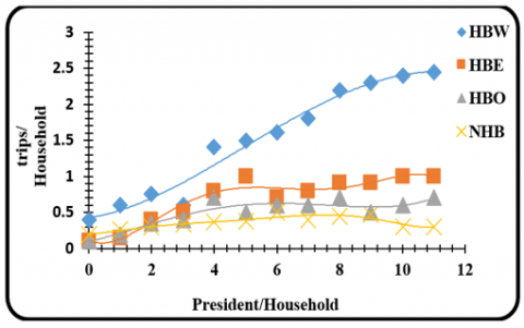
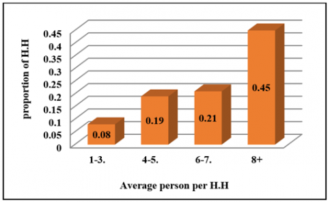
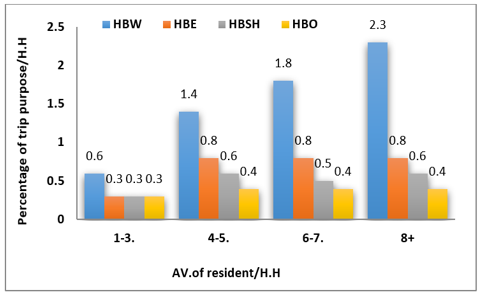
Trip Generation by Households (H.H): The trips generated by households are classified as Home-Based (HB) and Non-Home-Based (NHB). Home-based trips have one end, either origin or destination, located at the home zone of the trip maker. If both ends of a trip are located in zones where the trip maker does not live, it is considered as a non-home-based trip [13]. For modelling, the study adopted the HB trips which had been categorized as four purposes which are: Home Based Work (HBW), Home Based education (HBE), Home Based Shopping (HBSH) and Home Based Other (HBO), which gave a satisfying data can adopt at model development. The Non-Home Based (NHB) had been excluded because the number of forms of their that obtained from Home Interview Survey (HIS) was too few and it cannot represent the individual movement. Thus, "Category Analysis" [9, 14] had been used to obtain trip rate by splitting the household at each traffic zone for categories according to the average person per household. Two curves had been developed. One, reveals the relation between the rate of household size and proportion of population. While, the other, reveals the relation between the rate of trips /trip purpose and household size as shown in Figure 2 and Figure 3 respectively. The rate of the household is extracted from dropping the value of H.H size for zone on a curves in Figure 2 to obtain the rate of H.H/ H.H size as illustrated in Figure 4
Sequentially, Figure 3 shows the relationship between the rate of trips/trip destination and the size of the household; the analysis will extrapolate the average trip rate according to trip purpose as Figure 5.
Figure 2. Relation between the rate of household size and proportion of a person
Figure 3. Relation between the rate of trips /trip purpose and household size
Figure 4. Rate of H.H/ H.H size
Figure 5. Average trip rate according to trip purpose
The trip production in any zone depending on H.H and average trip rate. For estimation rate of household trip production, it’s multiplying the average household trip rate according to the purpose for each household size by its percentage in Figure 3 then have been multiply by the total number of the household at each zone. Thus bellow the estimating of trip production for zone No.1.
Average H.B.W rate=0.6×0.08+1.4×0.19+1.8×0.21+2.3×0.45=1.7
Since the No. of (HBW) trip for zone 1 = 1.7× (No. of H.H for zone 1 = 948[10])=1.7×948 = 1612 trip
The same procedure has been applied for estimating all trips purpose for all city as shown in Table 1.
Table 1. Trips Production by purpose at all zones for the base year
|
Zone No. |
|||||||||||||||||||||||
|
Trip purpose |
1 |
2 |
3 |
4 |
5 |
6 |
7 |
8 |
9 |
10 |
11 |
12 |
13 |
14 |
15 |
16 |
17 |
18 |
19 |
20 |
21 |
22 |
sum |
|
HBW |
1612 |
3752 |
3457 |
23823 |
34149 |
42037 |
86150 |
89378 |
95029 |
56050 |
47127 |
56061 |
93166 |
62281 |
19819 |
34196 |
48144 |
25199 |
75071 |
21143 |
33417 |
3752 |
95295 |
|
HBE |
796 |
1581 |
576 |
513 |
759 |
1311 |
1632 |
1929 |
1470 |
1638 |
1242 |
1272 |
1389 |
1377 |
729 |
735 |
957 |
1125 |
237 |
939 |
858 |
951 |
23574 |
|
HBSH |
588 |
273 |
237 |
576 |
474 |
744 |
519 |
552 |
1629 |
399 |
264 |
381 |
438 |
723 |
453 |
309 |
681 |
624 |
267 |
312 |
537 |
291 |
10884 |
|
HBO |
408 |
243 |
237 |
279 |
309 |
603 |
261 |
231 |
327 |
156 |
186 |
318 |
513 |
399 |
252 |
189 |
339 |
534 |
135 |
309 |
321 |
291 |
6528 |
|
SUM |
3404 |
3039 |
1479 |
2139 |
2373 |
3546 |
3711 |
4596 |
5439 |
3120 |
2643 |
3180 |
3654 |
3585 |
2514 |
2370 |
3120 |
3288 |
1029 |
2403 |
2679 |
2643 |
63735 |
Table 2. Rate of trip attraction/purpose
|
Trip purpose |
HBW |
HBED |
HBO |
NHB |
SUM |
|
Rate / total trips |
42% |
37.2% |
14.8% |
6% |
100% |
Table 3. Trip Attraction for 2020
|
Trip Attraction |
Zone No |
||||||||||||||||||||||
|
1 |
2 |
3 |
4 |
5 |
6 |
7 |
8 |
9 |
10 |
11 |
12 |
13 |
14 |
15 |
16 |
17 |
18 |
19 |
20 |
21 |
22 |
Sum |
|
|
Attraction |
19412 |
8398 |
7046 |
3758 |
21479 |
5396 |
2359 |
2454 |
2930 |
1066 |
822 |
5396 |
4205 |
3513 |
11019 |
1846 |
1263 |
716 |
2096 |
2321 |
2995 |
4459 |
114949 |
|
HBW 42% |
8153 |
3527 |
2959 |
1578 |
9021 |
2266 |
991 |
1031 |
1231 |
448 |
345 |
2266 |
1766 |
1475 |
4628 |
775 |
530 |
300 |
880 |
975 |
1258 |
1873 |
8153 |
|
HBED 37.2% |
7221 |
3124 |
2621 |
1398 |
7990 |
2007 |
878 |
913 |
1090 |
397 |
306 |
2007 |
1564 |
1307 |
4099 |
687 |
470 |
266 |
780 |
863 |
1114 |
1659 |
42761 |
|
HBSH 14.8% |
2873 |
1243 |
1043 |
556 |
3179 |
799 |
349 |
363 |
434 |
158 |
122 |
799 |
622 |
520 |
1631 |
273 |
187 |
106 |
310 |
344 |
443 |
660 |
17012 |
|
HBO 6% |
1165 |
504 |
423 |
225 |
1289 |
324 |
142 |
147 |
176 |
64 |
49 |
324 |
252 |
211 |
661 |
111 |
76 |
43 |
126 |
139 |
180 |
268 |
6897 |
Otherwise, trip attraction, it is a typical practice to utilize total models as linear regression conditions [15] for trip attractions. The dependent variable for these total models is trip attraction. While, the independent variables and according to Figure 5, the trip work had been got the largest use, therefor the study adopted just the employment variable for the building attraction model which represent zonal total values. But it is recommended to expand the model attraction by adopting other variables (e.g. educational and recreation) for reaching more accuracy outcomes. Thus, the study reached for relation at Eq. (3) below:
Aj=1.689Ej+586 (3)
where, Aj is the trip attraction for zone j and Ej is the zonal employment j.
The correlation coefficient of the model achieved 80%, and the rate of trip per No. of trips purpose it's going to excreted results as shown in Table 2.
The rate above at Table 2 will be duplicated for all zones to obtain the trip attraction within the city for the base year. Table 3 reveals the estimation of a trip attraction of Nassiriyah city for the base year of 2020.
The number of the trips generated between all of the zones of origin i and all of the zones of destination j should be equal to the total end of trip generated in the zone of origin for any destination zone, similar declarations can be mad. These are recognized as the constraints on flow conservation are given as follows:
$\sum_{j=1}^{n} T \mathrm{ij}=O i$ (4)
$\sum_{i=1}^{n} T \mathrm{ij}=D j$ (5)
Based on Eq. (1) will be obtained:
$\sum_{j=1}^{n}(\mathrm{Ki} \mathrm{Lj} . \mathrm{Oi} . \mathrm{Dj} f(\mathrm{dij}))=O i$ (6)
$\sum_{i=1}^{n}(\mathrm{Ki} \mathrm{Lj} .O \mathrm{i} . \mathrm{Dj} f(\mathrm{dij}))=D j$ (7)
By arranging the equations above obtained the following equations:
$\operatorname{Lj} D j \sum_{j=1}^{n}(\mathrm{Ki} .$ Oi $f(\mathrm{dij}))=D j$ (8)
$K i O i \sum_{j=1}^{n}(\mathrm{Lj} . \operatorname{Dj} f(\mathrm{dij}))=O i$ (9)
Finally, the study is reaching to two equations as bellow:
$\mathrm{Ki}=\frac{1}{\sum_{j=1}^{n}(\mathrm{Lj}. \mathrm{Dj} f(\mathrm{dij}))}$ (10)
$\mathrm{Lj}=\frac{1}{\sum_{i=1}^{n}(\mathrm{Ki} . \mathrm{Oi} \mathrm{f}(\mathrm{dij}))}$ (11)
Another step, the impedance function takes different formulas of functions [13], so for investigate the study very important step is calculating Impedance function. As the literature, the impedance function takes different formulas of functions [13], so for investigate the study distance had been using the following Equation as an impedance function. The impedance function takes different formulas of functions [13], so for investigate the study distance had been using the following Equation as an impedance function.
$f(d i j)=(d i-j)^{m} \times e^{-x \cdot d i j}$ (12)
where:
di-j = distance between zone i and j, x, m = constant
The matrix of distance had been estimated depending on a plan of the Nassiriyah city on scale (1: 100000). At this stage, program used to distribute the trips on zones inside and at outside of the city, upon on Gravity Model and for calculating all variables which show in steps (a, b and c). While the constant (x, m) found by two stages, one supposes limit values for (m, x) as illustrate in bellow formula:
$f(d i-j)=d i-j^{1.6} \times e^{-0.78 d i-j}$ (13)
By substituting the value of (d) from the distance matrix to find the constant (Ki, Lj) so suppose K1=1 and using Eq. (11) will obtain a value of the parameter of Lj. Then entering this value in Equation 10 for reaches to a new value of Ki. Thus, the iterative process continues until the values of Ki Thus, the iterative process continues until the values of Ki, Lj converge of the next iterative process, thus obtaining the values of (Ki, Lj), at last going to calculate trip distribution matrix (Ti-j) and compare it with the observed trip matrix for a base year that's lead to estimate the ratio of error as follows:
R. Error $=\sum \mathrm{i} \sum \mathrm{j} \frac{\mathrm{Ti}-\mathrm{j} . \mathrm{T}^{\wedge} \mathrm{i}-\mathrm{j}}{\mathrm{Ti}-\mathrm{j}}$ (14)
where, $\mathrm{T}^{\wedge} \mathrm{i}-\mathrm{j}$ is the calculating value and Ti-j is the observed value.
At comparative the ratio of error in the formula above with the opposite values that lead to determining the need to change the constant value (m, x) at impedance function. The value of m and x at range (1.8-2.5) and (0.5-0.75) respectively, these steps represent the second stage in the correction. The dependability of model investigation at estimates the constant value in the model as (Ki, Lj, m, x) according to permitted data for the base year. When comparing with observation value, can select the model for future prediction.
At Stage 2, The study used Fratar’s method for distributing the trips. It is one of Growth factored methods, the advantage of this method, its take all growth factors for different areas at distribution trips. The study used the Eq. (2) as mention earlier in section 3. The model involved many periods to reach for a matrix, which the different at its been convergence in value of trips that attracted to all zones at the base year with the value of trip attraction at the target year. The growth factor has been determining as greater than 1 and less than 1.2.
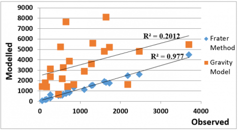
The outcomes of trip distribution models are usually calibrated by contrast between O-D trips observed verses O-D trips modelled so, the findings indicate that in most volume groups up to 4000 trips with the gravity model, the Fratar system forecasts compare best with the O-D assignments as illustrated in Figure 6.
Figure 6 shows a linear relationship. It is showing the slopes and R2 for each model. Thus, it shows that Frater's method was accurate for the base year of the study area according to the value of the coefficient of determination was 0.977, it is representing a high value to explain the strength between the observed and modelled trips. While the Gravity model among the zones did not give accurate results here the coefficient of determination was 0.2012.
Figure 6. Calibration of models
As mention in section 3. The outcomes of trip distribution models are usually calculated by the contrast between modelled O-D trips and observed ones. More precisely, this paper will analyze the effects of the calibrated models using three parameters, as follows [16]:
1- The root means square error percentage (RMSE percentage), a metric for the average of individual O-D pairs, can be determined as follows:
$\% \mathrm{RMSE}=\frac{\mathrm{RMSE}}{\mathrm{t}-} \times 100$ (15)
where, $\mathrm{RMSE}=\sqrt{\frac{\sum_{i j} t i j-T i j}{X}}$, $\mathrm{t}-=\frac{\sum_{i j}(t i j)}{X}$, tij is observed trips between zone i and zone j, Tij is estimated trips between zone i and zone j and X is number of observed non-zero O-D pairs.
2- Percentage of mean absolute change per trip (%MADPT) that can be calculated as follow:
$\%$ MADPT $=\frac{\sum_{i j}|t i j+T i j|}{\sum_{i j} t i j} \times 100$ (16)
3- Mean absolute change per cell (MADPC) that can be calculated as follows:
$\% M A D P C=\frac{\sum_{i j}|t i j+T i j|}{n} \times 100$ (17)
So, the three parameters above gave the result as a Table 4 bellow:
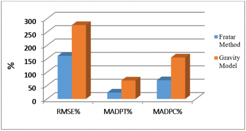
Table 4. Statically result of Fratar and Gravity mode
|
Model |
Parameters |
||
|
RMSE% |
MADPT % |
MADPC% |
|
|
Gravity |
276 |
69 |
155 |
|
Fratar |
161 |
24 |
70 |
Table 5. Modelled trip matrix for the base year 2020
|
Zone No |
Destination |
|||||||||||||||||||||||
|
Origin |
|
1 |
2 |
3 |
4 |
5 |
6 |
7 |
8 |
9 |
10 |
11 |
12 |
13 |
14 |
15 |
16 |
17 |
18 |
19 |
20 |
21 |
22 |
sum |
|
1 |
846 |
134 |
134 |
150 |
22 |
20 |
76 |
57 |
547 |
113 |
143 |
466 |
39 |
20 |
47 |
18 |
33 |
320 |
655 |
31 |
326 |
480 |
4607 |
|
|
2 |
688 |
90 |
90 |
69 |
26 |
14 |
31 |
59 |
300 |
37 |
128 |
111 |
141 |
25 |
95 |
46 |
31 |
276 |
446 |
46 |
220 |
479 |
3458 |
|
|
3 |
1275 |
86 |
86 |
64 |
31 |
21 |
33 |
72 |
235 |
43 |
131 |
96 |
24 |
29 |
44 |
417 |
59 |
131 |
589 |
224 |
1506 |
443 |
5638 |
|
|
4 |
1600 |
131 |
131 |
74 |
55 |
39 |
34 |
56 |
1015 |
46 |
300 |
70 |
17 |
17 |
39 |
85 |
77 |
280 |
2248 |
2900 |
667 |
1004 |
10814 |
|
|
5 |
1729 |
128 |
128 |
173 |
29 |
24 |
31 |
46 |
317 |
33 |
187 |
224 |
9 |
11 |
20 |
207 |
20 |
373 |
726 |
243 |
1357 |
261 |
6200 |
|
|
6 |
1636 |
85 |
85 |
147 |
24 |
13 |
38 |
96 |
781 |
57 |
122 |
113 |
16 |
9 |
27 |
278 |
43 |
1470 |
1338 |
72 |
131 |
410 |
7077 |
|
|
7 |
2185 |
87 |
87 |
70 |
21 |
16 |
29 |
57 |
967 |
68 |
56 |
345 |
22 |
27 |
33 |
100 |
1431 |
78 |
1140 |
52 |
85 |
672 |
7610 |
|
|
8 |
261 |
86 |
86 |
44 |
26 |
9 |
20 |
17 |
130 |
122 |
60 |
134 |
21 |
20 |
20 |
497 |
564 |
68 |
740 |
40 |
39 |
98 |
3101 |
|
|
9 |
559 |
56 |
56 |
52 |
31 |
11 |
25 |
29 |
503 |
65 |
68 |
91 |
31 |
74 |
1654 |
143 |
59 |
113 |
744 |
20 |
329 |
512 |
5160 |
|
|
10 |
261 |
38 |
38 |
29 |
16 |
13 |
16 |
17 |
134 |
115 |
24 |
72 |
43 |
711 |
56 |
60 |
18 |
44 |
540 |
26 |
55 |
122 |
2405 |
|
|
11 |
131 |
64 |
64 |
48 |
26 |
11 |
18 |
35 |
116 |
116 |
29 |
121 |
367 |
43 |
30 |
135 |
26 |
59 |
261 |
24 |
40 |
74 |
1773 |
|
|
12 |
1307 |
147 |
147 |
117 |
12 |
17 |
27 |
59 |
837 |
141 |
81 |
1654 |
16 |
17 |
46 |
102 |
27 |
108 |
880 |
60 |
173 |
421 |
6306 |
|
|
13 |
649 |
116 |
116 |
85 |
27 |
22 |
34 |
53 |
1129 |
86 |
419 |
134 |
13 |
29 |
99 |
143 |
38 |
450 |
774 |
261 |
306 |
742 |
5656 |
|
|
14 |
3697 |
89 |
89 |
60 |
47 |
11 |
22 |
35 |
663 |
246 |
43 |
341 |
21 |
30 |
57 |
134 |
44 |
74 |
726 |
56 |
74 |
930 |
7474 |
|
|
15 |
2468 |
113 |
113 |
37 |
22 |
21 |
42 |
59 |
2731 |
122 |
73 |
61 |
9 |
8 |
31 |
46 |
20 |
146 |
531 |
30 |
555 |
551 |
7829 |
|
|
16 |
728 |
83 |
83 |
89 |
29 |
17 |
64 |
982 |
190 |
99 |
42 |
55 |
21 |
35 |
29 |
69 |
47 |
186 |
551 |
16 |
254 |
215 |
3873 |
|
|
17 |
576 |
40 |
40 |
26 |
25 |
29 |
507 |
46 |
134 |
147 |
103 |
100 |
14 |
24 |
30 |
74 |
31 |
42 |
711 |
46 |
172 |
325 |
3261 |
|
|
18 |
169 |
26 |
26 |
31 |
39 |
447 |
21 |
24 |
118 |
60 |
24 |
57 |
7 |
7 |
27 |
42 |
24 |
37 |
76 |
20 |
94 |
76 |
1420 |
|
|
19 |
456 |
43 |
43 |
57 |
2341 |
26 |
40 |
43 |
313 |
137 |
68 |
86 |
11 |
13 |
18 |
59 |
21 |
56 |
442 |
47 |
115 |
245 |
4661 |
|
|
20 |
55 |
17 |
17 |
885 |
14 |
13 |
13 |
30 |
94 |
27 |
24 |
42 |
8 |
7 |
4 |
5 |
8 |
56 |
57 |
39 |
21 |
39 |
1451 |
|
|
21 |
516 |
2152 |
2152 |
46 |
56 |
26 |
70 |
61 |
453 |
363 |
98 |
276 |
11 |
16 |
35 |
65 |
29 |
85 |
563 |
5 |
55 |
170 |
4044 |
|
|
22 |
1097 |
113 |
113 |
37 |
57 |
33 |
43 |
60 |
450 |
161 |
61 |
204 |
22 |
26 |
29 |
99 |
42 |
221 |
840 |
42 |
245 |
332 |
3463 |
|
|
sum |
22862 |
3894 |
3894 |
2360 |
2947 |
822 |
1204 |
1962 |
12130 |
2373 |
2252 |
4822 |
852 |
1166 |
2440 |
2794 |
2661 |
4642 |
15547 |
6787 |
326 |
8545 |
107282 |
|
Figure 7. Statical result for Fratar and Gravity model
Table 4 shows the values for the various model formulations of the above-mentioned error measures. The graphical presentation of these outcomes is shown in Figure 7. It can be noticed that the best trip distribution model is the Fratar, based on Table 4 and Figure 7. With a significant relative variance, the Fratar Approach showed the lowest values of the three error steps. The percent RMSE of gravity forms improved by Fratar by about 39 percent with respect to the percent MADPT value, the improvement was about 61 compared to the gravity model.
Accordingly, a trip distribution matrix was built based on the results of the Fratar method, as shown in Table 5.
(1) First of all, the process of data collection and survey conducting for each zone needs a long time and cost with large stresses. Hence it must be planned before starting, as well as it’s required an institution work. Data that obtained wasn't an accuracy but, it gave acceptable information.
(2) To outline the main point of modelling trip distribution, it is depending on building trip generation model which represent a firstly studying that had been conducted in all Nasiriyah city take on the household characteristics. The model of attraction that used in modelling had been represented by the relationship between the number of trips and number of employees (Ej) at the same zone represented by Eq. (3). The model is a simplified the purpose of study, as well as it gives a good result. But recommend to inter other variables for this equation such as educational and recreation. The model attraction can use for redistribution of employment on the zones of the city for secure balance between zones to reduce traffic volume on the Central Business District network (CBD).
(3) For the modelling trip distribution, Model of Fratar proved its possibility of using it in forecasting for Al Nasiriyah city, because this method is successfully used for a homogenous growth areas. As well as in updating the data of the survey of the origin and destination of trips that collected recently, although this method does not care for rapid growth patterns. The Fratar's method has been used, it gave satisfactory results.
(4) Gravity model did not investigate a real result because Nassiriyah city is a medium-sized so as the city is not experiencing rapid changes, as well as the distances between its sectors, do not constitute an obstacle for any trip.
(5) For the gravity model, the best calibrated friction factor functions are as follows:
$f(d i-j)=d i-j^{1.6} \times e^{-0.78 d i-j}$
(6) The developing Matrix of trip distribution can be adopted for enhancing transportation network.
Finally, the study recommended:
(1) Adopt future academic studies interested with trip distribution according to its purpose take into the model split and traffic assignment to suggest the alternative for a quote strategy of the transportation system.
(2) The issue of outing conveyance is non-direct nature therefore the study recommends to use Neural Networks (NN) is appropriate for tending to the non-direct issues.
[1] Goel, S., Singh, J.B., Sinha, A.K. (2012). Trip distribution model for Delhi urban area using genetic algorithm. International Journal of Computer Engineering Science (IJCES), 2(3): 1-8.
[2] de Grange, L., Fernández, E., de Cea, J. (2010). A consolidated model of trip distribution. Transportation Research Part E: Logistics and Transportation Review, 46(1): 61-75. https://doi.org/10.1016/j.tre.2009.06.001
[3] Rasouli, M. (2014). Trip distribution modelling using neural network. Doctoral dissertation, Curtin University.
[4] Mathew, T.V., Rao, K.K. (2006). Introduction to Transportation Engineering. Civil Engineering–Transportation Engineering. IIT Bombay, NPTEL ONLINE.
[5] Salter, R.J. (1996). Highway Traffic Analysis and Design. Macmillan International Higher Education.
[6] Yaldi, G., Taylor, M.A., Yue, W.L. (2011). Forecasting origin-destination matrices by using neural network approach: A comparison of testing performance between back propagation, variable learning rate and Levenberg-Marquardt algorithms. In Australasian Transport Research Forum.
[7] Herijanto, W., Thorpe, N. (2005). Developing the singly constrained gravity model for application in developing countries. Journal of the Eastern Asia Society for Transportation Studies, 6: 1708-1723. https://doi.org/10.11175/easts.6.1708
[8] Abdel-Aal, M.M.M. (2014). Calibrating a trip distribution gravity model stratified by the trip purposes for the city of Alexandria. Alexandria Engineering Journal, 53(3): 677-689. https://doi.org/10.1016/j.aej.2014.04.006
[9] Chatterjee, A., Venigalla, M.M. (2004). Travel demand forecasting for urban transportation planning. Handbook of Transportation Engineering. ISBN: 978-0071391221.
[10] Population Statistics Directorate - City of Nassiriyah - Central Statistical Organization-household for Neighborhoods Housing for the city of Nassiriyah, 2017.
[11] de Dios Ortúzar, J., Willumsen, L.G. (2011). Modelling Transport. John Wiley & Sons.
[12] de Dios Ortúzar, J., Willumsen, L.G. (1996). Modeling Transport, Second edition. John Wiley & Sons Ltd., England.
[13] Kadiyali, L.R., Lal, N.B. (2011). Traffic Engineering and Transport Planning. Khanna Publishers, 9th Reprint.
[14] Garber, N.J., Hoel, L.A. (2014). Traffic and Highway Engineering. Cengage Learning.
[15] Papacostas, C.S., Prevedouros, P.D. (1993). Transportation Engineering and Planning. 3rd ed, Prentice, Hall of India, Private Limited.
[16] Transportation Planning Center (TRANSPLAN). (1999). Study of calibration the strategic national transportation models. Transport Planning Authority, Ministry of Transportation, Egypt.