Leena Samantaray | Sabonam Hembram | Rutuparna Panda*
© 2020 IIETA. This article is published by IIETA and is licensed under the CC BY 4.0 license (http://creativecommons.org/licenses/by/4.0/).
OPEN ACCESS
The exploitation capability of the Harris Hawks optimization (HHO) is limited. This problem is solved here by incorporating features of Cuckoo search (CS). This paper proposes a new algorithm called Harris hawks-cuckoo search (HHO-CS) algorithm. The algorithm is validated using 23 Benchmark functions. A statistical analysis is carried out. Convergence of the proposed algorithm is studied. Nonetheless, converting color breast thermogram images into grayscale for segmentation is not effective. To overcome the problem, we suggest an RGB colour component based multilevel thresholding method for breast cancer thermogram image analysis. Here, 8 different images from the Database for Research Mastology with Infrared images are considered for the experiments. Both 1D Otsu’s between-class variance and Kapur's entropy are considered for a fair comparison. Our proposal is evaluated using the performance metrics – Peak Signal to Noise Ratio (PSNR), Feature Similarity Index (FSIM), Structure Similarity Index (SSIM). The suggested method outperforms the grayscale based multilevel thresholding method proposed earlier. Moreover, our method using 1D Otsu’s fitness functions performs better than Kapur’s entropy based approach. The proposal would be useful for analysis of infrared images. Finally, the proposed HHO-CS algorithm may be useful for function optimization to solve real world engineering problems.
optimizer, Harris Hawks optimization, cuckoo search, multilevel thresholding, thermogram image analysis
Breast cancer is most common among women. Over 2.1 million women get affected each year, and the death rates are highly related to the breast cancer [1]. It is the second most common cancer in women after lungs cancer. Breast Cancer mostly begins in the ducts or lobules after uncontrolled growth of the cells. Breast cancer can spread to distant organs, so an early treatment is required. Cancer is a disease with multiple factors, so advanced screening of the breasts is required for analysis of the tumor formation. Breast cancer can be classified in several stages, the initial stage, which is known as DCIS (ductal carcinoma in situ), the growth of cells is limited in ducts. In the next stage, the formation of tumor occurs, and also has a small group of cancer cells. When the size of the tumor grows, it spreads to lymph nodes and distant organs such as bones, liver, brain or lungs.
Advanced screening of breasts is required for analysis of tumor formation as an extra aid to a radio-physicist. There are various Medical imaging techniques used for early analysis of breast cancer, Such as Breast Ultrasound (Sonogram), Magnetic Resonance (MRI), Thermography, Mammography, Positron Emission Tomography (PET), Computed Tomography (CT), Integrated PET/CT, MRI and PET, Ultrasound and MRI.
Mammography is one of the popular diagnostic techniques used for the detection of breast cancer. Mammography involves exposure to X-ray radiation on the human body. Due to the exposure to radiation, there is a possibility of further cancer cell growth. Sometimes Mammography, Breast MRI and Breast Ultrasound show “false-positive” results, in which the person needs an additional test or even more. This could lead to another mammogram or a different test.
On the other hand, thermography is a clinical procedure where a thermal camera captures the infrared radiation of the human body at controlled room temperature and produces the digital thermal images. A body emits infrared radiation above absolute zero temperature. A thermal image shows the temperature variations of the body. The infrared radiation emitted by the surface of the body has wavelength ranges from 0.8µm to 10 µm. Thermography is a non-invasive process, no exposure to radiations and does not involve in compression of breast tissues [2]. Thermography provides information on the growth of cancer cells before the formation of a tumour. No radiation is involved as the temperature variation of the body provides vascular activity information.
Image Segmentation Partitions images into regions into homogeneous classes. For image segmentation, several techniques have been studied throughout the years. Multilevel thresholding is the easiest method in image segmentation. In color images, multilevel thresholding partitions, images into different classes based on threshold levels of each R, G, B histogram components. The thresholding based segmentation method is divided into parametric and non-parametric. Note that the parametric method calculates the probability density function of each class, whereas the nonparametric measure class variance, entropy to get the optimal threshold values [3]. Due to the computational complexity of the parametric approach, nonparametric methods are used. Various optimization techniques are used in multilevel thresholding using nonparametric approaches to get the best threshold values. Segmentation of medical images is popular in recent years as it is helpful for analysis of a particular part of the body.
In this work, a new optimization technique called Harris Hawks-Cuckoo Search (HHO-CS) is investigated. The Harris Hawks optimizer is found more popular for function optimization. However, its exploitation capability is limited, thereby not yielding to optimal or near optimal solutions. This has motivated us to incorporate the exploitation capability of the cuckoo search strategy. This is the real motivation behind the investigation of the proposed HHO-CS algorithm. Two different objective functions are used for a comparison. The suggested algorithm is used to obtain the optimal threshold values to segment colour thermogram images. The effectiveness of HHO-CS algorithm is validated with a set of 23 Benchmark functions and compared with Harris Hawks optimization [4] and Cuckoo Search algorithm [5]. For multilevel thresholding of thermogram images, experiments are performed based on Otsu’s between-class variance and Kapur's entropy as the fitness functions. Our proposed HHO-CS technique is evaluated based on the performance metrics – peak signal to noise ratio (PSNR), Feature similarity index (FSIM), Structure Similarity Index (SSIM). Results of objective function values, threshold levels of RGB component are also evaluated.
Converting colour thermal images into grayscale images makes it a difficult task to extract features due to poor contrast, low visual perception. Therefore, it is necessary to perform full colour image processing of the clinical images for research support. For the past few years, many optimization techniques are used to perform segmentation to get better quality segmented images. This has motivated us to investigate a method to segment colour thermogram images. Results are presented using 1D Otsu’s objective function and Kapur’s entropy.
Organization of the paper is as follows: Section 2 discusses the related work. The proposed HHO-CS algorithm is presented in Section 3. The methodology is discussed in Section 4. Results are presented in Section 5. Conclusions are given in Section 6.
Díaz-Cortés et al. [6] in 2018 presented multilevel thresholding of Breast Thermal images using Dragonfly algorithm. The Segmentation of grayscale breast thermal images is performed by using the energy curve of images as an input. The colour Segmentation of satellite images using nature-inspired optimization algorithms are proposed by Bhandari et al. [7]. The performance of the algorithms was performed based on Otsu’s between-class variance and Kapur’s entropy as the objective functions. The Kapur’s entropy based objective function has better performance and the Cuckoo search algorithm was found to be more efficient for Colour segmentation of satellite images.
He and Huang [8] presented an efficient krill herd (EKH) optimization technique for multilevel thresholding of colour images using Otsu’s method, Kapur and Tsallis entropy as the objective functions. The efficient krill herd (EKH) algorithm shows better performance as compared to the krill herd algorithm (KH). Electro-magnetism optimization (EMO) algorithm based multilevel thresholding is presented by Oliva et al. [9]. The Otsu’s and Kapur's entropy criterion used as objective functions and the histogram of images are taken as the input. Oliva et al. [3] presented a hybrid Artificial Bee colony-Salp Swarm algorithm (ABC-SSA), for image segmentation. The hybrid approach performs better than ABC, SCA, SSO, SSA algorithms in a multilevel thresholding problem using Kapur’s entropy as the objective function. Multilevel thresholding of Satellite images proposed by Pare et al. [10] using optimization techniques WDO, BFO, FA, ABC, DE and PSO by taking energy curves of image as an input. The objective functions based on Kapur’s entropy, Tsallis entropy and Otsu’s method are used. The Kapur’s entropy based DE techniques produces better segmented images.
Multilevel thresholding using WDO and CS was proposed by Bhandari et al. [11] using Kapur’s entropy as the objective function. Multilevel thresholding using various Optimization techniques are reported in the studies [12-15]. Horng et al. [16] presented multilevel thresholding based on honey bee mating optimization using the cross entropy as the objective function. Bhandari et al. [17] proposed a modified artificial Bee colony (MABC) optimizer for multilevel thresholding of satellite images through maximization of Otsu’s between-class variance, Kapur’s and Tsallis entropy. The MABC algorithm produces better segmented images as compared to ABC method.
2.1 Harris Hawks Optimization
A nature-inspired Optimization algorithm called “Harris-Hawks optimization”algorithm was proposed by Heidari et al. in 2019. The Harris-hawks optimization technique is inspired by the hunting strategy of Harris-hawks and escaping of prey. The Harris-hawks catch prey by a “Surprise Pounce” or also known as“Seven kills”strategy. The Harris-hawks optimization technique also features exploration and exploitation phase [4].
2.1.1 Exploration phase
The exploration phase of HHO algorithm consists of two strategies to detect the prey (Rabbit) by perching randomly on some locations, taking an equal chance q (in each perching plan), the perch based on the position of other hawks. The location of the rabbit is known as $\begin{equation}X_{\text {rabbit }}\end{equation}$. The rabbit location for the condition q< 0.5 described in Eq. (1). When q $\begin{equation}\geq\end{equation}$ 0.5, hawks roost on random high trees inside their range of location.
$\begin{equation}
X(t+1)=\left\{\begin{array}{l}
X_{\text {rand}}-r_{1}\left|X_{\text {rend}}(t)-2 r_{2} X(t)\right|, q \geq 0.5 \\
\left(X_{\text {rabbit}}(t)-X_{m}(t)\right)-r_{3}\left(L B+r_{4}(U B-L B)\right), q<0.5
\end{array}\right.
\end{equation}$ (1)
where, The term X(t+1) represents updated position of Hawks in each iteration, $\begin{equation}X_{\text {rabbit}}(t)\end{equation}$ is the postion of rabbit, $\begin{equation}X_{\text {rand}}(t)\end{equation}$ is the position of Hawks chosen randomly, LB is the lower bound, UB is the upper bound, and $\begin{equation}X_{m}(t)\end{equation}$ is the average position of hawks. Random numbers $\begin{equation}\mathrm{r}_{1}, \mathrm{r}_{2}, \mathrm{r}_{3}, \mathrm{r}_{4}\end{equation}$ are used to explore different regions of Search space for the Hawks. The equation for the average position of hawks is given by:
$\begin{equation}
X_{m}(t)=\frac{1}{N} \sum_{i=1}^{N} X_{i}(t)
\end{equation}$ (2)
where, $\begin{equation}\mathrm{X}_{\mathrm{i}}(\mathrm{t})\end{equation}$ and N represents the location of each Hawk in iteration t and number of Hawks, respectively. The transition from the Exploration Phase to Exploitation Phase occurs depending on the Perching strategy of Hawks on escaping prey (Rabbit). The initial energy $\begin{equation}\mathrm{E}_{0}\end{equation}$ The value ranges from -1 to 1 for every iteration t. When the value of $\begin{equation}\mathrm{E}_{0}\end{equation}$ decreases from 0 to -1, it signifies a weakening of the prey. In case the value of $\begin{equation}\mathrm{E}_{0}\end{equation}$ increases from 0 to 1, it signifies strengthening of the prey. The escaping energy of the Prey also a key factor in the transition, which is modelled as:
$\begin{equation}
E=2 E_{0}\left(1-\frac{t}{T}\right)
\end{equation}$ (3)
2.1.2 Exploitation phase
The Hawks perform the “Surprise Pounce” strategy to catch the prey. There is also an escaping factor ‘r’ of the prey, where the value of r is greater than 0.5 signify higher chance of escape and less than or equal to 0 signify lower chance of escape of the rabbit. There are different phases of exploitation of prey based on the escaping factor and energy of the prey. The exploitation phases are shown in Figure 1.
Figure 1. Exploitation phases of HHO
a. Soft Besiege
The Hawks perform Soft Besiege based on Rabbit’s energy. The position of hawks for soft Besiege models as below.
$\begin{equation}
X(t+1)=\Delta X(t)-E / J X_{\text {rabbit}}(t)-X(t) /
\end{equation}$ (4)
$\begin{equation}
\Delta X(t)=X_{\text {rabbit}}(t)-X(t)
\end{equation}$ (5)
where, “J” is known as“Jump strength”of the Rabbit.
b. Hard Besiege
When the Rabbit is fagging, the hawks perform “Surprise Pounce” tactics, when the escaping factor value “r” is greater than or equal to 0.5 and the escaping energy is less than 0.5. For each iteration, the positions of hawks are updated using the equation.
$\begin{equation}
X(t+1)=X_{\text {rabbit}}(t)-E|\Delta X(t)|
\end{equation}$ (6)
where, E is the energy.
c. Soft Besiege with progressive rapid dives
In Case of Escaping energy greater than or equal to 0.5 and the escaping factor less than 0.5 of the rabbit, the hawks perform soft besiege with progressive rapid dives. In this condition, the rabbit has sufficient energy to outflow). The Levy flight movement of Hawks depends on the zig-zag motion of the rabbit [6]. The Hawks update their position concerning the movements of the rabbit. The equations for this strategy can be described as below:
$\begin{equation}
Y=X_{\text {rabbir}}(t)-E\left|J X_{\text {rabbit}}(t)-X(t)\right|
\end{equation}$ (7)
$\begin{equation}
Z=Y+S \times L F(D)
\end{equation}$ (8)
$\begin{equation}
L F(x)=0.01 \times \frac{u \times \sigma}{|v|^{\frac{1}{\beta}}}
\end{equation}$ (9)
where,
$\begin{equation}
\begin{array}{l}
\sigma=\left(\frac{\Gamma(1+\beta) \times \sin \left(\frac{\pi \beta}{2}\right)}{\Gamma\left(\frac{1+\beta}{2}\right) \times \beta \times 2^{\left(\frac{\beta-1}{2}\right)}}\right)^{\frac{1}{\beta}} \\
X(t+1)=\left\{\begin{array}{l}
Y, F(Y)<F(X(t)) \\
Z, F(Y)<F(X(t))
\end{array}\right.
\end{array}
\end{equation}$ (10)
Note that LF is the Levy flight.
d. Hard Besiege with progressive rapid dives
When Escaping energy is less than 0.5 and escaping factor is less than 0.5, the rabbit is completely exhausted and has low-level energy, the Hawks perform hard besiege with rapid dives to catch the rabbit. In this stage, the hawks successfully catch the rabbit. The Levy flight method is also used in this phase. The equation for the position of hawks, for each iteration, is given below:
$\begin{equation}
X(t+1)==\left\{\begin{array}{ll}
Y, & \text { if } F(Y)<F(X(t)) \\
Z, & \text { if } F(Z)<F(X(t))
\end{array}\right.
\end{equation}$ (11)
$\begin{equation}
Y=X_{\text {rabbit}}(t)-E \mid J X_{\text {rabbit}}(t)-X_{m}(t)
\end{equation}$ (12)
$\begin{equation}
Z=Y+S \times L F(D)
\end{equation}$ (13)
2.2 Cuckoo search optimization
Nature-inspired Cuckoo Search optimization was proposed by Yang and Deb in 2009 [5]. The Cuckoo Search algorithm is based on the brooding parasitism of Cuckoo birds as they use another host bird’s nest for breeding. The phases of the cuckoo search algorithm are described below
1) A cuckoo bird lays one egg at a time and pass down to another bird’s nest;
2) The best nests with good quality eggs are carried over to the next generations;
3) The number of host nests is fixed, and the host bird can discover an egg with a probability of $\begin{equation}p_{a}\end{equation}$ ∈ [0,1]. Interestingly, the host bird can either throw the egg or abandon the nest immediately. The number of nests “n” and“ $\begin{equation}p_{a}\end{equation}$ ”are replaced with new solutions.
The mathematical equation, for each iteration, is modelled as below.
$\begin{equation}
x_{i}^{(t+1)}=x_{i}^{(t)}+\alpha \oplus \text {Lévy}(\lambda)
\end{equation}$ (14)
The equation for the levy flight mechanism is given below.
$\begin{equation}
\text { Lévy } \sim u=t^{-\lambda},(1<\lambda \leq 3)
\end{equation}$ (15)
where, ‘u’ is the variable and ‘$\begin{equation}\lambda\end{equation}$’ is a constant.
Harris Hawks Optimization technique performs good exploration tactics to catch the prey to reach a global best solution, whereas the weak exploitation capability of hawks signifies a higher chance of getting into local optima. To enhance the performance of HHO, the exploitation capability of Cuckoo search mechanism is inherited here. The location of hawks is updated by:
$\begin{equation}
\begin{array}{l}
X(t+1)= \\
\left\{\begin{array}{c}
X_{\text {rand}}(t)-r_{1}\left|X_{\text {rand}}(t)-2 r_{2} X(t)\right|+\alpha \oplus \text {Lévy}(\lambda), q \geq 0.5 \\
\left.X_{\text {rabbit}}(t)-X_{m}(t)\right)-r_{3}\left(L B+r_{4}(L B+(U B-L B))+\alpha \oplus\right. \text {Lévy}(\lambda) \\
q<0.5,|E| \geq 1
\end{array}\right.
\end{array}
\end{equation}$ (16)
Figure 2. Flow diagram of HHO-CS
The flow diagram of HHO-CS method is displayed in Figure 2.
Table 1. Parameter settings
|
Algorithm |
Parameter |
Value |
|
HHO-CS |
N $\begin{equation} $\begin{equation} |
30 0.25 1.5 |
|
HHO |
N |
30 |
Table 2. Results of benchmark functions ( $\begin{equation}f_{1}\end{equation}$ - $\begin{equation}f_{13}\end{equation}$ ), with 30 dimensions
|
Function |
|
HHO-CS |
HHO |
|
f 1 |
Avg Std Min Max |
8.8674E-95 4.8557E-94 4.5074E-115 2.6596E-93 |
1.6694E-94 6.9584E-94 1.9980E-121 3.6163E-93 |
|
f 2 |
Avg Std Min Max |
5.9147E-49 2.3401E-48 3.3248E-59 1.2151E-47 |
1.3618E-49 7.2705E-49 3.4078E-59 3.9850E-48 |
|
f 3 |
Avg Std Min Max |
2.6211E-72 1.4357E-71 1.2370E-98 7.8634E-71 |
8.4362E-76 3.3003E-75 4.5853E-99 1.5885E-74 |
|
f 4 |
Avg Std Min Max |
2.5076E-49 9.4690E-49 6.2383E-58 5.0141E-48 |
8.8527E-49 3.6383E-48 4.5837E-58 1.9624E-47 |
|
f 5 |
Avg Std Min Max |
0.0290 0.0524 3.9738E-5 0.2504 |
0.0172 0.0339 1.7375E-5 0.1741 |
|
f 6 |
Avg Std Min Max |
1.0566E-04 1.2169E-04 9.8245E-08 4.9675E-04 |
1.2869E-04 1.5884E-04 4.6149E-07 6.6066E-04 |
|
f 7 |
Avg Std Min Max |
1.4913E-04 2.0653E-04 1.0482E-05 8.6431E-04 |
1.7717E-04 1.4357E-04 3.0423E-06 6.6621E-04 |
|
f 8 |
Avg Std Min Max |
-1.2486E+04 45.2858 -1.2569E+04 -1.2350E+04 |
-1.2562E+04 40.0058 1.2569E+04 1.2350E+04 |
|
f 9 |
Avg Std Min Max |
0 0 0 0 |
0 0 0 0 |
|
f 10 |
Avg Std Min Max |
8.8818E-16 1.47E+02 8.8818E-16 8.8818E-16 |
8.8818E-16 1.47E+02 8.8818E-16 8.8818E-16 |
|
f 11 |
Avg Std Min Max |
0 0 0 0 |
0 0 0 0 |
|
f 12 |
Avg Std Min Max |
5.9841E-06 9.2809E-06 1.4347E-08 3.4656E-05 |
1.1300E-05 2.2354E-05 7.8338E-09 1.1656E-04 |
|
f 13 |
Avg Std Min Max |
7.0957E-05 1.2754E-04 2.4497E-08 6.3517E-04 |
8.1648E-05 9.4889E-05 5.8620E-09 3.5137E-04 |
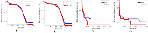
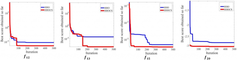
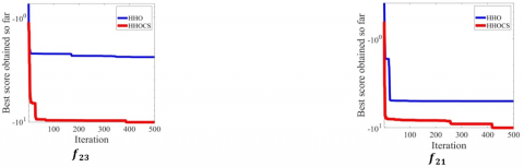
Figure 3. Convergence curves of HHO-CS and HH
Table 3. Results of benchmark functions ($\begin{equation}f_{14}-f_{23}\end{equation}$)
|
Function |
|
HHO-CS |
HHO |
|
f 14 |
Avg Std Min Max |
1.5585 1.2876 0.9980 5.9288 |
1.3280 0.9466 0.9980 5.9288 |
|
f 15 |
Avg Std Min Max |
3.4236E-04 2.9925E-05 3.0756E-04 4.4702E-04 |
3.8963E-04 2.6287E-04 3.0771E-04 1.8000E-03 |
|
f 16 |
Avg Std Min Max |
-1.0316 6.78E-16 -1.0316 -1.0316 |
-1.0316 6.78E-16 -1.0316 -1.0316 |
|
f 17 |
Avg Std Min Max |
0.3979 2.54E-06 0.3979 0.3979 |
0.3979 2.54E-06 0.3979 0.3979 |
|
f 18 |
Avg Std Min Max |
3 0 3 3 |
3 0 3 3 |
|
f 19 |
Avg Std Min Max |
-3.6028 1.4095 -3.8628 -3.8599 |
-3.8590 0.0061 -3.8628 -3.8333 |
|
f 20 |
Avg Std Min Max |
-3.1250 0.0726 -3.2605 -2.9690 |
-3.0913 0.0988 -3.2836 -2.8111 |
|
f 21 |
Avg Std Min Max |
-5.5267 1.4608 -10.0063 -5.0028 |
-5.1375 1.0277 -10.0464 -2.6226 |
|
f 22 |
Avg Std Min Max |
-5.2484 0.9042 -10.0360 -5.0679 |
-5.2495 0.9097 -10.0658 -5.0685 |
|
f 23 |
Avg Std Min Max |
-5.4583 1.2722 -10.4055 -5.1106 |
-5.3041 0.9876 -10.5332 -5.1076 |
Benchmark Function Optimization
To test the effectiveness of HHO-CS, HHO, and CS algorithms, a set of 23 standard benchmark functions including unimodal, multimodal, multimodal with fixed dimension functions ( $\begin{equation}f_{1}-f_{23}\end{equation}$ ) are taken for a minimization problem. The unimodal functions are used to test the exploitation capability of optimizers and the multimodal functions are used to test the exploration ability. The unimodal functions also signify the ability to reach the global best while the performance of the multimodal functions shows the local optima avoidance. The dimension size is set to 30. The population size N is 30 and the maximum iteration is 500. All the algorithms are run in MATLAB R2018 having an Intel Core i5-8265U CPU clocked at 1.60GHz with 4GB RAM, with windows 10 operating system. The parameter settings are shown in Table 1. The results of an Average (Avg), Standard deviation (Std), Minima (Min) and Maxima (Max) of 30 runs of each benchmark functions are shown in Table 2&3. The boldface letters indicate the best results. The convergence curves are shown in Figure 3.
In summary, the proposed HHO-CS algorithm performs better than the HHO for the multimodal test functions. However, the performance of our method is similar to that of the HHO for some of the functions. Nevertheless, the suggested algorithm ensures a better convergence, because of its enhanced exploitation capability.
Multilevel thresholding of color thermogram images is solved using the RGB histogram as the input, considering that the color images contain more information, better visual perception of the human eye with contrary to grayscale images, where we cannot see the temperature variations. The multilevel thresholding technique is used to get better results.
4.1 Otsu’s between class variance
The bi-level and multilevel thresholding of images based on the between class variance was first proposed by Otsu [18]. Bi-level thresholding and multilevel thresholding separate images into classes when the maximum variance is calculated. This method considers histogram of an image as an input. The probability distribution of intensity levels of R, G, B channel is obtained. The optimal threshold values are obtained for each channel of the colour image. The mathematical representation is given below
$\begin{equation}
\sigma^{2}=\sum_{k=1}^{n t} \sigma_{k}=\sum_{k=1}^{n t} \omega_{k}\left(\mu_{k}-\mu_{\tau}\right)^{2}
\end{equation}$ (17)
$\begin{equation}
\mu_{\star}=\sum_{i=t h k}^{t h_{k+1}-1} \frac{k P E_{i}}{\omega_{i}\left(t h_{i}\right)}
\end{equation}$ (18)
where,
$\begin{equation}
\omega_{k}=\sum_{i=t h k}^{t h k+1-1} P E_{i}
\end{equation}$ (19)
$\begin{equation}
f_{\text {otsu}}(t h)=\max \left(\sigma^{2}(t h)\right), 0 \leq \text { th } \leq \mathrm{L}-1
\end{equation}$ (20)
where, $\begin{equation}\sigma^{2}\end{equation}$ is the variance, µ is the mean.
4.2 Kapur’s entropy
Kapur’s entropy method measures the entropy of different classes of an image. To segment colour images, the Kapur’s entropy maximizes the entropy and obtain optimal threshold values of each R, G, B channel. The probability distribution of intensity levels of each R, G, B channel is used to measure the entropy criterion. Segmentation of Colour images performed by maximizing Kapur’s entropy, which is taken as the objective function [19]. The mathematical formulations for Kapur’s entropy are
$\begin{equation}
f_{\text {Kapur}}(t h)=\max \left(\sum_{k=1}^{n t} H_{k}\right)
\end{equation}$ (21)
where, entropy of each class is calculated by
$\begin{equation}
H_{k}=\sum_{i=t h k}^{t h k+1-1} \frac{P E_{i}}{\omega_{k}} \ln \left(\frac{P E_{i}}{\omega_{k}}\right)
\end{equation}$ (22)
In summary, the proposed Harris Hawks-Cuckoo Search Optimizer (Eq. (16)) is used to optimize the fitness functions shown in Eq. (20) (Otsu’s method) and Eq. (21) (Kapur’s method). It is reiterated that the optimum threshold values are obtained through the maximization.
The multilevel colour thermogram image thresholding method is implemented using both Otsu’s between-class variance and Kapur’s entropy as the fitness functions. The proposed HHO-CS, CS and HHO algorithms are implemented to get optimal results. The multilevel colour thermogram image thresholding method is shown in Figure 4.
Figure 4. Multilevel thresholding of thermal images
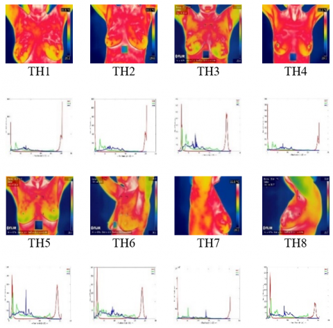
The benchmark images are displayed in Figure 5. The experiments are based on a set of 8 different images acquired from the Database for Research Mastology with Infrared images [20]. The images are captured using a FLIR SC-620 Thermal Camera. The selected images and their respective histogram plots are described in Figure 5. For experimental purposes, images with size 341 x 256 are taken.
The population size and the maximum number of iterations of each algorithm are set to 30 and 500, respectively. The Lower bound (LB) and upper bound (UB) of the algorithm is set to 0 to 255. The performance of the algorithms is evaluated, which is composed of 20 runs of the same algorithm using a specific image and calculating the average of objective function values, PSNR, SSIM and FSIM [21-24].
Figure 5. Benchmark images and their respective histograms
5.1 Benchmark images
The Peak Signal to noise ratio (PSNR) is a widely used performance metric for measuring the quality of the original image with the reconstructed images. Structure Similarity Index (SSIM) and Feature Similarity index (FSIM) quality metric measure the similarity between the original image and the output segmented image. SSIM specify quality degradation due to data processing. All experiments are performed on MATLAB R2018a with 4GB RAM on an Intel core i5 CPU clocked at 1.6 GHz frequency.
5.2 Experiment 1: Based on Otsu’s between class variance
Optimal threshold values are obtained using HHO-CS algorithm and presented in Table 4. Objective function values and PSNR values obtained from HHO-CS and HHO algorithms using Otsu’s between class variance are displayed in Table 5. Remarkable differences are found. It is observed that the suggested HHO-CS method outperforms as compared to HHO. Similarly, a significant improvement over the HHO algorithm is seen with respect to the PSNR values. The reason could be the enhanced exploitation capability of HHO-CS method to get the best solutions. For instance, an improvement of 3% in PSNR value is seen in the test image sample TH1 with threshold level K=4 (see Table 5). The SSIM and FSIM values obtained from HHO-CS and HHO algorithms using Otsu’s between-class variance are shown in Table 6. Interestingly, the suggested technique has shown better values (for SSIM and FSIM) than HHO.
Table 4. Threshold values obtained using HHO-CS algorithm
|
Image |
K |
HHO-CS |
||
|
|
|
R |
G |
B |
|
TH1 |
2 |
137,239 |
110,210 |
82,163 |
|
3 |
141,176,230 |
60,153,182 |
62,130,149 |
|
|
4 |
44,58,113,145 |
44,102,160,230 |
46,86,135,250 |
|
|
5 |
145,191,196,197,254 |
61,87,168,173,255 |
83,98,152,196,236 |
|
|
TH2 |
2 |
138,236 |
82,88 |
81,190 |
|
3 |
108,212,228 |
62,60,140 |
51,86,118 |
|
|
4 |
101,155,176,255 |
93,130,167,228 |
46,94,185,198 |
|
|
5 |
112,180,183,224,255 |
83,96,126,200,247 |
82,128,137,239,254 |
|
|
TH3 |
2 |
125,229 |
102,238 |
83,86 |
|
3 |
136,147,180 |
81,151,215 |
63,110,196 |
|
|
4 |
140,188,212,249 |
59,91,140,243 |
63,104,195,248 |
|
|
5 |
32,153,155,190,249 |
83,96,97,103,231 |
60,76,86,164,196 |
|
|
TH4 |
2 |
148,203 |
95,174 |
77,90 |
|
3 |
100,189,222 |
56,130,217 |
52,107,108 |
|
|
4 |
104,164,194,250 |
110,148,175,251 |
80,114,190,215 |
|
|
5 |
106,111,184,249,254 |
64,69,88,123,217 |
58,88,64,65,104 |
|
|
TH5 |
2 |
137,138 |
101,209 |
75,88 |
|
3 |
113,141,201 |
60,134,141 |
47,63,126 |
|
|
4 |
155,162,172,254 |
112,146,147,219 |
84,94,202,215 |
|
|
5 |
130,165,192,217,253 |
86,166,174,187,218 |
76,96,176,209,220 |
|
|
TH6 |
2 |
128,137 |
47,100 |
85,147 |
|
3 |
117,134,206 |
56,131,209 |
71,138,166 |
|
|
4 |
130,143,170,254 |
118,120,126,216 |
60,117,202,244 |
|
|
5 |
66,185,195,199,245 |
94,107,119,148,208 |
55,84,93,162,247 |
|
|
TH7 |
2 |
139,184 |
93,97 |
56,85 |
|
3 |
115,124,214 |
63,136,158 |
59,61,129 |
|
|
4 |
219,237,241,251 |
110,167,184,232 |
91,120,243,246 |
|
|
5 |
114,118,142,250,255 |
78,138,186,191,240 |
29,68,92,133,207 |
|
|
TH8 |
2 |
125,139 |
100,126 |
92,130 |
|
3 |
97,190,243 |
43,64,131 |
54,83,169 |
|
|
4 |
125,156,162,253 |
126,134,218,233 |
94,95,131,213 |
|
|
5 |
141,156,159,213,247 |
93,115,182,238,253 |
21,63,98,241,247 |
|
Table 5. Comparison of objective function and PSNR values obtained from HHO-CS and HHO algorithms using Otsu’s between-class variance
|
|
|
OBJECTIVE FUNCTION |
PSNR |
||
|
Images |
K |
HHO-CS |
HHO |
HHO-CS |
HHO |
|
TH1 |
2 3 4 5 |
1.3864 E+04 1.4623 E+04 1.7680 E+04 1.9050 E+04 |
1.3829E+04 1.4581E+04 1.7483E+04 1.8744E+04 |
55.0114 62.7343 69.6979 74.3875 |
53.4132 62.5010 67.6563 73.3842 |
|
TH2 |
2 3 4 5 |
1.5874 E+04 1.6509 E+04 1.9470 E+04 2.0844 E+04 |
1.5860E+04 1.6499E+04 1.8832E+04 1.9810E+04 |
55.3194 62.4648 66.3321 72.0098 |
54.1919 61.3768 65.7321 71.8845 |
|
TH3 |
2 3 4 5 |
1.2160 E+04 1.3104 E+04 1.8422 E+04 2.0441 E+04 |
1.2133E+04 1.3012E+04 1.7919E+04 1.8662E+04 |
55.3793 62.1599 65.2385 68.4839 |
53.9000 60.9659 64.2440 66.8464 |
|
TH4 |
2 3 4 5 |
1.6818 E+04 1.7437 E+04 2.1086 E+04 2.2654 E+04 |
1.6807E+04 1.7369E+04 1.9552E+04 2.1593E+04 |
56.1415 58.5895 64.3450 66.0842 |
54.938 55.1351 60.9177 64.0399 |
|
TH5 |
2 3 4 5 |
1.2864 E+04 1.3962 E+04 1.8368 E+04 2.0739 E+04 |
1.2858E+04 1.3833E+04 1.7688E+04 1.9943E+04 |
56.2041 57.7679 59.3859 62.8876 |
55.5316 56.0270 58.7054 61.4830 |
|
TH6 |
2 3 4 5 |
1.4484 E+04 1.5325 E+04 2.0903 E+04 2.2077 E+04 |
1.4467E+04 1.5185E+04 2.0314E+04 2.1627E+04 |
56.5041 58.1370 64.2811 66.2539 |
55.0818 57.5004 63.2488 65.4236 |
|
TH7 |
2 3 4 5 |
1.8836 E+04 1.9405 E+04 2.2614 E+04 2.5290 E+04 |
1.8825E+04 1.9340E+04 2.1881E+04 2.3362E+04 |
57.6207 63.8870 65.7686 66.2036 |
55.0971 62.9271 63.9271 65.7404 |
|
TH8 |
2 3 4 5 |
1.4799 E+04 1.5705 E+04 2.1482 E+04 2.2905 E+04 |
1.4757E+04 1.5658E+04 2.1221E+04 2.2280E+04 |
57.6318 64.2626 67.8773 69.2639 |
56.5587 64.2060 67.5404 68.6456 |
Table 6. Comparison of SSIM and FSIM values obtained from HHO-CS and HHO algorithms using Otsu’s between class variance
|
|
|
SSIM |
FSIM |
||
|
Images |
K |
HHO-CS |
HHO |
HHO-CS |
HHO |
|
TH1 |
2 3 4 5 |
0.7342 0.7829 0.8280 0.8604 |
0.6967 0.7355 0.8181 0.8523 |
0.7515 0.8029 0.8140 0.8396 |
0.7486 0.7992 0.8110 0.8347 |
|
TH2 |
2 3 4 5 |
0.7114 0.8079 0.8501 0.9109 |
0.6912 0.7904 0.8483 0.8976 |
0.7586 0.7946 0.8267 0.8438 |
0.7170 0.7781 0.8231 0.8362 |
|
TH3 |
2 3 4 5 |
0.7281 0.7964 0.8248 0.8787 |
0.7060 0.7784 0.8174 0.8653 |
0.7676 0.8025 0.8238 0.8449 |
0.7468 0.7970 0.8258 0.8418 |
|
TH4 |
2 3 4 5 |
0.6699 0.8010 0.8324 0.8963 |
0.6662 0.7934 0.8292 0.8714 |
0.7840 0.8170 0.8344 0.8570 |
0.7698 0.8106 0.8210 0.8359 |
|
TH5 |
2 3 4 5 |
0.7401 0.8007 0.8591 0.8729 |
0.7238 0.7952 0.8470 0.8667 |
0.7419 0.7739 0.8255 0.8996 |
0.7361 0.7680 0.8137 0.8811 |
|
TH6 |
2 3 4 5 |
0.7287 0.7728 0.8421 0.8899 |
0.7207 0.7702 0.8388 0.8890 |
0.7676 0.8272 0.8310 0.8485 |
0.7533 0.8158 0.8237 0.8442 |
|
TH7 |
2 3 4 5 |
0.7009 0.7765 0.8461 0.8914 |
0.6941 0.7507 0.8422 0.8884 |
0.7920 0.8189 0.8335 0.8628 |
0.7823 0.8153 0.8266 0.8445 |
|
TH8 |
2 3 4 5 |
0.7194 0.8192 0.8476 0.8777 |
0.6839 0.8119 0.8426 0.8701 |
0.7921 0.8213 0.8418 0.8550 |
0.7907 0.8177 0.8356 0.8521 |
5.3 Results of HHO-CS algorithm using Otsu’ between-class variance
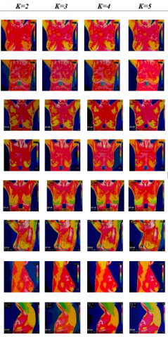
Segmented results of HHO-CS algorithm using Otsu’s method is shown in Figure 6. Both the low contrast and high contrast visual features are retained. The quality of the output is implicit. The proposed method may attract radio physicists to use it as an additional tool for diagnosis.
Figure 6. Results of HHO-CS algorithm using Otsu’s method
5.4 Experiment 2: Based on Kapur’s entropy
Optimal threshold values, obtained using HHO-CS algorithm, are displayed in Table 7. Objective function values and PSNR values obtained from HHO-CS and HHO methods using Kapur’s entropy are presented in Table 8. Profound differences are seen. It is observed that the suggested HHO-CS method performs better than the HHO. Similarly, a significant improvement over the HHO algorithm is seen with respect to the PSNR values. The reason could be the enhanced exploitation capability of HHO-CS algorithm to achieve the best solutions. Our method has shown consistently better PSNR values than HHO (see Table 8). The SSIM and FSIM values obtained from HHO-CS and HHO algorithms using Kapur’s entropy are shown in Table 9. Interestingly, our method has shown better values (for the SSIM and FSIM) than the HHO.
Table 7. Threshold values of HHO-CS
|
Images |
K |
HHO-CS |
||
|
|
|
R |
G |
B |
|
TH1 |
2 |
227,234 |
42,179 |
233,252 |
|
3 |
190,229,255 |
125,145,200 |
51,71,189 |
|
|
4 |
132,137,187,247 |
15,104,136,210 |
32,42,141,233 |
|
|
5 |
98,115,202,203,212 |
3,75,102,115,186 |
25,112,158,188,232 |
|
|
TH2 |
2 |
239,255 |
106,206 |
25,191 |
|
3 |
208,235,255 |
16,132,247 |
35,88,238 |
|
|
4 |
166,200,218,250 |
141,216,245,251 |
38,68,199,228 |
|
|
5 |
116,153,168,190,250 |
98,103,177,200,215 |
42,60,80,176,198 |
|
|
TH3 |
2 |
221,227 |
230,239 |
186,255 |
|
3 |
126,230,244 |
87,137,154 |
21,33,131 |
|
|
4 |
129,156,204,223 |
80,84,187,227 |
126,190,222,227 |
|
|
5 |
104,138,143,228,255 |
54,82,130,169,223 |
16,36,58,205,238 |
|
|
TH4 |
2 |
227,255 |
47,120 |
169,255 |
|
3 |
137,158,236 |
82,121,254 |
62,120,190 |
|
|
4 |
136,194,209,224 |
51,57,80,249 |
41,46,144,182 |
|
|
5 |
164,166,239,245,254 |
5,51,59,114,118 |
85,164,176,187,207 |
|
|
TH5 |
2 |
236,249 |
87,254 |
44,148 |
|
3 |
189,203,255 |
31,229,244 |
191,219,233 |
|
|
4 |
188,202,219,253 |
115,147,239,250 |
3,40,132,252 |
|
|
5 |
99,160,176,197,250 |
49,82,124,231,250 |
70,85,109,133,226 |
|
|
TH6 |
2 |
212,229 |
45,117 |
119,245 |
|
3 |
137,168,203 |
115,129,218 |
3,73,153 |
|
|
4 |
105,123,200,250 |
77,92,138,250 |
74,133,136,252 |
|
|
5 |
147,196,209,230,252 |
19,35,66,133,164 |
36,69,188,222,243 |
|
|
TH7 |
2 |
250,252 |
179,242 |
178,243 |
|
3 |
215,220,254 |
3,102,158 |
126,150,157 |
|
|
4 |
104,184,237,246 |
33,49,156,208 |
5,68,117,245 |
|
|
5 |
150,151,200,209,251 |
25,159,180,196,229 |
9,31,34,106,191 |
|
|
TH8 |
2 |
233,249 |
251,252 |
30,163 |
|
3 |
219,225,233 |
14,142,219 |
69,100,124 |
|
|
4 |
179,198,211,242 |
35,63,83,129 |
3,131,181,246 |
|
|
5 |
89,139,166,202,234 |
26,79,102,114,251 |
27,34,74,149,159 |
|
Table 8. Comparison of objective function values and PSNR obtained from HHO-CS and HHO algorithms using Kapur’s entropy
|
|
|
OBJECTIVE FUNCTION |
PSNR |
||
|
Image |
K |
HHO-CS |
HHO |
HHO-CS |
HHO |
|
TH1 |
2 3 4 5 |
25.3967 36.4699 42.8620 50.2350 |
23.8390 34.0063 39.4868 48.4930 |
48.8151 53.1784 55.0468 59.3109 |
48.3047 52.8795 54.5950 58.2001 |
|
TH2 |
2 3 4 5 |
25.8282 32.0311 40.5143 50.2481 |
25.6571 31.2724 40.2226 48.3490 |
53.1854 58.6532 62.7254 65.2311 |
52.9000 58.1990 62.0969 65.6008 |
|
TH3 |
2 3 4 5 |
26.7611 33.3907 41.5988 51.4126 |
26.6938 32.1520 40.8171 50.8451 |
50.1649 52.0191 56.6610 60.1033 |
48.5777 51.0425 56.1281 59.7543 |
|
TH4 |
2 3 4 5 |
26.8261 32.5919 37.2682 46.2737 |
23.7504 31.6829 37.0698 46.1896 |
53.8566 56.3193 61.9640 65.6875 |
52.0168 55.2586 61.7853 65.5550 |
|
TH5 |
2 3 4 5 |
27.6672 34.4082 40.0538 48.3672 |
27.1914 34.3798 39.3762 47.7147 |
50.1393 54.0606 58.6640 60.4075 |
48.6514 53.9827 57.6439 59.3283 |
|
TH6 |
2 3 4 5 |
26.9100 35.6760 44.2570 50.4478 |
23.9546 33.8006 40.7154 50.3543 |
50.3106 53.5330 62.0879 63.5159 |
46.0928 51.0713 55.1715 63.5070 |
|
TH7 |
2 3 4 5 |
25.7328 32.2351 41.8437 45.9847 |
25.5387 32.1220 41.7025 45.5572 |
50.1983 53.8161 58.3176 60.1012 |
50.1500 53.1795 57.5759 59.5965 |
|
TH8 |
2 3 4 5 |
25.8521 33.2082 40.5836 49.3672 |
25.4122 32.3197 39.5286 49.3606 |
48.1895 53.7797 58.8640 63.8921 |
47.3364 53.6042 57.9005 63.8803 |
Table 9. Comparison of SSIM and FSIM values from HHO-CS and HHO algorithms using Kapur’s entropy
|
|
|
SSIM |
FSIM |
||
|
Image |
K |
HHO-CS |
HHO |
HHO-CS |
HHO |
|
TH1 |
2 3 4 5 |
0.6241 0.6707 0.8155 0.8571 |
0.5798 0.6643 0.8028 0.8317 |
0.6870 0.7283 0.7510 0.7849 |
0.6632 0.7103 0.7496 0.7835 |
|
TH2 |
2 3 4 5 |
0.5481 0.7343 0.7836 0.8283 |
0.4899 0.6783 0.7482 0.8315 |
0.7122 0.7438 0.7630 0.7782 |
0.7084 0.7417 0.7583 0.7992 |
|
TH3 |
2 3 4 5 |
0.5980 0.7112 0.7358 0.8388 |
0.5208 0.6878 0.7033 0.8058 |
0.6772 0.7294 0.7668 0.7705 |
0.6623 0.7228 0.7655 0.7765 |
|
TH4 |
2 3 4 5 |
0.5191 0.7289 0.7478 0.8016 |
0.5160 0.6951 0.7266 0.7959 |
0.7124 0.7456 0.7621 0.7926 |
0.7100 0.7425 0.7617 0.7878 |
|
TH5 |
2 3 4 5 |
0.6818 0.7089 0.7416 0.8283 |
0.5718 0.6686 0.7132 0.8208 |
0.6790 0.7141 0.7284 0.7311 |
0.6773 0.6978 0.7165 0.7298 |
|
TH6 |
2 3 4 5 |
0.4988 0.6538 0.7238 0.7364 |
0.4164 0.5617 0.6815 0.7157 |
0.7221 0.7579 0.7994 0.8185 |
0.6941 0.7565 0.7879 0.8237 |
|
TH7 |
2 3 4 5 |
0.4523 0.6513 0.7897 0.7911 |
0.4510 0.5336 0.6850 0.7208 |
0.7920 0.8193 0.8335 0.8628 |
0.7823 0.8189 0.8266 0.8445 |
|
TH8 |
2 3 4 5 |
0.4331 0.6004 0.7162 0.7819 |
0.3654 0.4711 0.5864 0.6146 |
0.7909 0.8213 0.8418 0.8550 |
0.7921 0.8177 0.8356 0.8521 |
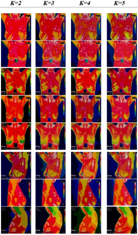
Figure 7. Results of HHO-CS algorithm using Kapur’s entropy
Segmented results of HHO-CS algorithm using Kapur’s entropy is shown in Figure 7. Both the low contrast and high contrast visual features are retained.
From this study, it is believed that the 1D Otsu’s between class variance method outperforms 1D Kapur’s entropy based technique. Because, infrared images, mostly have low contrast features. Therefore, between class variance helps us to compute optimal threshold values for separating different classes. It seems that the between class variance information is more than the entropy information in thermograms. In summary, the suggested multilevel colour image thresholding technique is useful for thermogram image analysis.
Unlike early multilevel thresholding method reported in the breast thermogram analysis, based on the gray-level images, the suggested method uses R, G, B colour components. The suggested technique is useful for the breast thermogram analysis. Results using the colour images may assist the clinicians, as an extra support, in the breast thermogram analysis. Nevertheless, the proposed HHO-CS optimizer helps us to compute optimal values for colour image thresholding. The exploitation capability of the HHO is enhanced, because the exploitation feature of CS is integrated in the system. Profound differences are observed while studying the convergence curves presented in this paper. The suggested HHO-CS performs better than both the HHO and CS optimizers. The speed of convergence is implicit (see Figure 3). The method has shown its ability to extract both the low and high resolution visual features, because all three colour components are used. The quality of the visual results is explicit (from Figure 6, 7). From Tables 4-6, it is observed that the RGB components based thresholding method using Otsu’s objective function is better than the Kapur’s entropy based approach; the reason is that the former fitness function could preserve more details. Therefore, the suggested RGB component based method using Otsu’s between class variance may be suitable for pathological investigations. To figure out other merits, our method is faster and more accurate. It is re-iterated that the proposed technique may attract the use of low cost and portable infrared cameras for analysis of breast thermograms. The proposal would be useful for analysis of other infrared images together with a clinical study. It is also believed that the suggested HHO-CS optimizer would be useful for function optimization to solve real world engineering problems.
[1] World Health Organization, Breast Cancer prevention, who.int/cancer/prevention/diagnosis-screening/breast-cancer/en/, accessed on 20 March 2020.
[2] Kennedy, D.A., Lee, T., Seely, D. (2009). A comparative review of thermography as a breast cancer screening technique. Integrative Cancer Therapies, 8(1): 9-16. https://doi.org/10.1177/1534735408326171
[3] Oliva, D., Elaziz, M.A., Hinijosa, S. (2019). Metaheurestic algorithms for Image segmentation: Theory and applications. Studies in Computational Intelligence. https://doi.org/10.1007/978-3-030-12931-6
[4] Heidari, A., Mirjalili, S., Faris, H., Aljarah, I., Mafarja, M., Chen, H. (2019). Harris hawks optimization: Algorithm and applications. Future Generation Computer System, 97: 849-872. https://doi.org/10.1016/j.future.2019.02.028
[5] Yang, X.S., Deb, S. (2009). Cuckoo search via Lévy flights. 2009 World Congress on Nature & Biologically Inspired Computing (NaBIC), Coimbatore, pp. 210-214. https://doi.org/10.1109/NABIC.2009.5393690
[6] Díaz-Cortés, M.A., Ortega-Sánchez, N., Hinojosa, S., Oliva, D., Cuevas, E., Rojas, R., Demin, A. (2018). A multi-level thresholding method for breast thermograms analysis using dragonfly algorithm. Infrared Physics & Technology, 93: 346-361. https://doi.org/10.1016/j.infrared.2018.08.007
[7] Bhandari, A.K., Kumar, A., Chaudhary, S., Singh, G.K. (2016). A novel color image multilevel thresholding based segmentation using nature inspired optimization algorithms. Expert Systems with Applications, 63: 112-133. https://doi.org/10.1016/j.eswa.2016.06.044
[8] He, L., Huang, S. (2020). An efficient krill herd algorithm for color image multilevel thresholding segmentation problem. Applied Soft Computing Journal, 89: 106063. https://doi.org/10.1016/j.asoc.2020.106063
[9] Oliva, D., Cuevas, E., Pajares, G., Zaldivar, D., Osuna, V. (2014). A multilevel thresholding algorithm using electromagnetism optimization. Neurocomputing, 139: 357-381. https://doi.org/10.1016/j.neucom.2014.02.020
[10] Pare, S., Kumar, A., Bajaj, V., Singh, G. (2019). A context sensitive multilevel thresholding using swarm based algorithms. IEEE/CAA Journal of Automanica Sinica, 6(6): 1471-1486. https://doi.org/10.1109/JAS.2017.7510697
[11] Bhandari, A.K., Singh, V.K., Kumar, A., Singh, G.K. (2014). Cuckoo search algorithm and wind driven optimization based study of satellite image segmentation for multilevel thresholding using Kapur’s entropy. Expert Systems with Applications, 41(7): 3538-3560. https://doi.org/10.1016/j.eswa.2013.10.059
[12] Ghamisi, P., Couceiro, M.S., Benediktsson, J.A., Ferreira, N.M.F. (2012). An efficien tmethod for segmentation of images based on fractional calculus and natural selection. Expert Systems with Applications, 39(16): 12407-12417. https://doi.org/10.1016/j.eswa.2012.04.078
[13] Ghamisi, P., Couceiro, M.S., Martins, F.M.L., Benediktsson, J.A. (2014). Multilevel image segmentation based on fractional-order Darwinian particle swarm optimization. IEEE Transactions on Geoscience and Remote Sensing, 52(5): 2382-2394. http://dx.doi.org/10.1109/TGRS.2013.2260552
[14] Hammouche, K., Diaf, M., Siarry, P. (2008). A multilevel automatic thresholding method based on a genetic algorithm for a fast image segmentation. Computer Vision and Image Understanding, 109(2): 163-175. https://doi.org/10.1016/j.cviu.2007.09.001
[15] Hammouche, K., Diaf, M., Siarry, P. (2010). A comparative study of various metaheuristic techniques applied to the multilevel thresholding problem. Engineering Applications of Artificial Intelligence, 23(5): 676-688. https://doi.org/10.1016/j.engappai.2009.09.011
[16] Horng, M.H. (2010). Multilevel minimum cross entropy threshold selection based on the honey bee mating optimization. Expert Systems with Applications, 37(6): 4580-4592. https://doi.org/10.1016/j.eswa.2009.12.050
[17] Bhandari, A.K., Kumar, A., Singh, G.K. (2015). Modified artificial bee colony based computationally efficient multilevel thresholding for satellite image segmentation using Kapur’s, Otsu and Tsallis functions. Expert Systems with Applications, 42(3): 1573-1601. http://dx.doi.org/10.1016/j.eswa.2014.09.049
[18] Otsu, N. (1979). A threshold selection method from Gray-level histograms. IEEE Transactions on Systems Man, Cybernetics, 9(1): 62-66. https://doi.org/10.1109/TSMC.1979.4310076
[19] Kapur, J.N., Sahoo, P.K., Wong, A.K.C. (1985). A new method for gray-level picture thresholding using the entropy of the histogram. Computer Vision, Graphics, and Image Processing, 29(3): 273-285. https://doi.org/10.1016/0734-189X(85)90125-2
[20] Database for Research mastology with Infrared images, visual lab, http://visual.ic.uff.br/dmi/, accessed on 20 March 2020.
[21] Horé, A., Ziou, D. (2010). Image quality metrics: PSNR vs. SSIM. 20th International Conference on Pattern Recognition, Istanbul, Turkey, pp. 2366-2369. https://doi.org/10.1109/ICPR.2010.579
[22] Zhang, L., Zhang, L., Mou, X., Zhang, D. (2011). FSIM: A feature similarity index for image quality assessment. IEEE Transactions on Image Processing, 20(8): 2378- 2386. https://doi.org/10.1109/TIP.2011.2109730
[23] Wunnava, A., Naik, M.K., Panda, R., Jena, B., Abraham, A. (2020). A differential evolutionary adaptive Harris hawks optimization for two dimensional practical Masi entropy-based multilevel image thresholding. Journal of King Saud University-Computer and Information Sciences, 1-14. https://doi.org/10.1016/j.jksuci.2020.05.001
[24] Wunnava, A., Naik, M.K., Panda, R., Jena, B., Abraham, A. (2020). An adaptive Harris hawks optimization technique for two dimensional grey gradient based multilevel image thresholding. Applied Soft Computing, 95: 1-35. https://doi.org/10.1016/j.asoc.2020.106526