Controlling the Nusselt Number in a TiO2/R134a Nano-refrigerant System

Khaled M.K. Pasha
© 2019 IIETA. This article is published by IIETA and is licensed under the CC BY 4.0 license (http://creativecommons.org/licenses/by/4.0/).
OPEN ACCESS
Experimental runs were performed to investigate the variation of the 'evaporator Nusselt number with the Reynolds number, the heat flux and the nano-Particles concentration in a refrigeration system. The used refrigerant is TiO2/R134a nano-fluid at different values of nano-particle concentration. Next, the refrigeration system was modified with an auxiliary evaporator and a control unit which will store the experimental results. These results will be used as a guide to distribute the mass and heat fluxes between the two evaporators. So, it is possible to control the Nusselt number and accordingly, to achieve a predetermined variation of the cooling behavior in more than one evaporator. The experimental results showed that, for all studied cases, the Nusselt number increased with the Reynolds number and the heat flux. The Nusselt number also increased with the Nano-Particle concentration up to the value of 0.5, and beyond this value, its enhancement started to deteriorate. When increasing the Reynolds Number by about 98 % the Nusselt number could be enhanced by about 67 %. Two correlations were suggested to fit the data of the Nusselt number, the heat flux, and the nano-particles concentration. This research work is a step towards the control of many cooling loads using one compressor.
refrigeration, nano-, evaporator, heat flux, reynolds
1.1 Theoretical investigation
For all refrigeration and HVAC systems, the heat transfer in the evaporator is an essential factor that assists the system performance and efficiency. One of the widely used refrigerants is R134a because it is widely accepted alternative refrigerant due to its low ozone depletion potential. It has a strong chemical polarity that allows the traditional mineral oil, mixed with it to be used as a lubricant and it is available and relatively less expensive. Many Researchers showed that, when using TiO2/ R134a nano-refrigerant in a refrigeration system, a considerable heat transfer enhancement occurs in its evaporator and, its compressors power is reduced too. Patil et al. [1] reviewed the thermal properties of nano-refrigerants and the energy consumption of its refrigerant systems. They reported that, when using 0.1 % mass fraction of TiO2 with POE, the energy consumption is reduced by 26.1 % of that in the case without TiO2. The freezing rate is slightly higher with the system with TiO2 as compared to the case of POE oil without TiO2. For many nano-particles that are dispersed in r134a, the effective thermal conductivity decreases with the particle size. But, it is still higher than the corresponding values of the cases where no nano-particles are added. The thermophysical and the heat transfer characteristics of TiO2-R134a nano-refrigerants were investigated during the boiling process by Sanukrishna et al. [2] They observed that the presence of TiO2 in a refrigerant can enhance the thermophysical properties and accordingly, the heat transfer coefficient could increase by 30.2 % when the particle concentration is 1.5 %. Yang and Hu [3] summarized the recent researches of the application of TiO2 nano-fluids. They concluded that, the thermal conductivity of nano-refrigerant increases with the volume fraction of TiO2. For 5 % volume fraction of TiO2 and temperature of 343 K, the enhancement in the thermal conductivity may reach the value of 30 %. The thermal conductivity also increases with temperature. At temperature 60 oC, the nano-refrigerant, which includes 4 % TiO2 nano-particles of average size 26 nm, attained 19 % enhancement in the thermal conductivity. Also, when using R134a and mineral oil with TiO2 nano-particles of size 50 nm and at concentration 10 g/L, the energy consumption of the system decreased by 7.43 %. In addition, using R134a and mineral oil with TiO2 nano-particles of size 50 nm and at concentration 0.1 % wt., the energy consumption of the system decreased by 26.1 %. Alawi et al. [4] investigated TiO2 nano-particles at very low concentrations with different refrigerants. They reported that the thermal conductivity is strongly temperature-dependent than that in the case of conventional refrigerant. Modifications to the thermophysical properties are the primary mechanism that affects heat transfer performance during flow boiling of nano-fluids. Increasing the thermal conductivity enhances the heat transfer, but, increasing the viscosity and surface tension reduces the heat transfer in nucleate boiling-dominated flows. A secondary mechanism appears when nano-particles fill up the micro-cavities on the test surface. It is also responsible for the decreased heat transfer and is a strong function of particle number density Kolekar et al. [5]. For a refrigeration system, many factors affect its thermal performance and its compressor power saving. Ajuka et al. [6] investigated the effects of evaporator temperature on the power consumption, coefficients of performance, exergetic efficiency and efficiency defects in the compressor, condenser, capillary tube and evaporator of the system. They used refrigerants R600a and LPG (R290/r600a: 50 %/ 50 %) at 0, 0.05, 0.15 and 0.3wt % concentrations of 15nm particle size of (TiO2) nano-lubricant, and (r134a). They concluded that, LPG + TiO2 (0.15wt %) and R600a + TiO2 (0. 15wt %) had the best performances with an average of 27.6% and 14.3% higher coefficient of Performance, 34.6 % and 35.15% lower power consumption. TiO2 nano-particles also increase the compatibility between the mineral oil and r134a, and the system that uses their mixture works safely with higher performance than that which uses r134a/POE alone. TiO2 nano-particles can enhance the heat transfer of the refrigerator system and also strengthen the lubrication capability of mineral oil, Yong et al. [7]. Adding TiO2 nano-particles at a concentration that ranges from 0.05 to 1 %, to R134 could enhance the heat transfer coefficient by a value of 50 % of that for the case pure fluid, Naas [8]. Using 0.1 % TiO2- mineral oil-R134a in a domestic Refrigerator has caused a maximum energy saving of (25 %), Javadi et al. [9]. The effect of 0.06 % TiO2 resulted in better saving than that of 0.1 % Al2O3. This reflects the deterioration of performance with the increase of TiO2 concentration and this result agrees with the conclusion of the present work. Subramani.N et al. [10] investigated the performance parameters of a vapor compression system with pure SUNISO 3GS oil and with different nano-lubricants. They reported that the freezing capacity was higher for TiO2 nano- lubricant compared with other studied cases. For the case of TiO2, they could achieve a reduction of 15.4 % in the compressor power. Padmanabhan and Palanisamy, [11] added 0.1 g of (TiO2 ) to each liter of Mineral oil, MO, that is mixed with (r134a), R436A and R436B. They reported that the total irreversibility (529, 588 and 570 W) at different process was better than the cases, where no TiO2 is used. Adelekana et al. [12] investigated varied mass charges of Liquefied Petroleum Gas (40 g, 50 g, 60 g and 70 g) with different (TiO2 ) nano-particle/ mineral oil concentrations (0.2 g/L, 0.4 g/L and 0.6 g/L nano-lubricants) in a R134a in a domestic refrigerator. They achieved a reduced compressor power input of about 21 W with the 70 g of LPG with either of 0.2 g/L or 0.4 g/L nano-lubricants. With 70 g of LPG using 0.6 g/L concentration of nano-lubricant, they could attain a cooling capacity index of 65 W. The highest COP of 2.8 was obtained with 40 g charge of LPG using 0.4 g/L concentration of nano- lubricant. Increasing the concentration of nano-particles (TiO2) in refrigerant results in an increase in the performances of the refrigeration system due to the decrease in the compressor work and the enhancement in the heat transfer rate. But for a system that works at high pressure in hot and dry climate condition, the performances of the condenser decreases. So, it is recommended to couple the vapor compression refrigeration system with an evaporative cooling pad. Dhamneya et al. [13] used this technique and reported a maximum increase in C.O.P. of about 51 %. Shengshan Bi et al. [14] experimentally investigated the nano-refrigerant TiO2-R600a in a domestic refrigerator using energy consumption test and freeze capacity test. They achieved an energy saving of 9.6% when they used TiO2 at a concentration of 0.5 g per each liter of r600a. They also obtained a better refrigerator performance than that of the pure R600 case. The idea of mixing more than nano-particle was investigated by Raghavalu et al. [15]. Nano-refrigerants Al2O3-Ethylene glycol oil and TiO2-Ethylene glycol oil were added to r134a. They reported that, when adding Al2O3 to R-134a, the COP of vapor compression refrigeration system improved by 12.08 % of that which does not use nano-particle. For the domestic refrigerator that uses LPG refrigerant with (TiO2) nano-particles dispersed in a mineral oil lubricant, the cooling capacity and COP of could be improved by 18.74–32.72 and 10.15–61.49 %, respectively. Furthermore, compressor power consumption and pressure ratio were decreased by about 3.20–18.1 and 2.33–8.45 %, respectively, Gill et al. [16]. TiO2 in the form of nano-particles may enhance the heat transfer coefficient. Also, TiO2 in the form of nano-layer can enhance the heat transfer coefficient. Ray et al. [17] investigated the pool boiling of R134a on flat copper surfaces that are fabricated with titanium dioxide (TiO2) thin film (TF) coating of thickness 100 nm and 200 nm. They reported that, with the 200 nm coating thickness, the heat transfer coefficient achieved the maximum enhancement over that of the case with uncoated cupper surface. This heat transfer coefficient enhancement is due to augmented roughness and increment of dynamic nucleation site density. Ray et al. [18] also investigated the pool boiling at 10 oC of R134a on flat copper surfaces that are coated with thin film of TiO2 nano-particles, and the film thicknesses are 100 nm, 200 nm, and 300 nm. They achieved a maximum of 87.5 % augmentation in the boiling heat transfer by the higher thickness of TiO2 coated surface than the bare copper surface. They interpreted the augmentation of heat transfer coefficient by the increase in micro/nano-porosity, active nucleation site density and surface area of the heating surface. The refrigerant R134 was tested with different nano-particles; Coumaressin and Palaniradja [19] investigated the refrigerant R134a with CuO nano-particle in a counterflow heat exchanger evaporator which is similar to that used in the present work. They evaluated the heat transfer coefficients for heat flux that ranged from 10 to 40 kW/m2 and used nano-particle concentrations that ranged from 0.05 to 1% and particle size from 10 to 70 nm. They reported that the heat transfer enhancement increased with the nano-particle concentration until a concentration of 0.55 %, and beyond this value, the enhancement rate started to deteriorate. This observation is similar to what was observed in the results of the present work. The effect of pressure on the heat transfer process attracted some researchers to investigate it. Cieśliński and Kaczmarczyk investigated the heat transfer coefficient during the pool boiling processes in a horizontal tube [20]. They tested two nano-fluids; water-Al2O3 and water-Cu at the concentration of 0.01 %, 0.1 %, and 1 % by weight. They established that increasing the operating pressure results in an enhancement in the heat transfer coefficient. Finally, not all refrigeration systems show enhancements in the heat transfer coefficient when using nano-refrigerants, but in some investigated cases, the performance deteriorates, and this agrees with the results of the present work. Kolekar et al. [5] obtained stable nano-fluids by mixing R134a with dispersions of surface-treated nano-particles TiO2 in polyol ester (POE) oil (RL22H and RL68H). They investigated the flow boiling over a range of mass flux from 100 to 1000 kg/m2 s, with a heat flux from 5 to 25 kw/m2, and vapor quality up to 1. They reported that the heat transfer coefficients decreased by 28 % TiO2/CO2 nano-fluids.
1.2 Objectives of the present work
In the present work, it is intended to accomplish two tasks;
Table 1 illustrates the different studied cases.
Table 1. TiO2 mass concentration, heat flux mass flux and reynolds number for the investigated cases
|
TiO2 Concentration, % |
Heat Flux, q, (Kw m-2) |
Reynolds number, Re |
|
0.05 |
33.17 |
4805 |
|
0.05 |
44.25 |
6387 |
|
0.05 |
56.53 |
8039 |
|
0.05 |
67.5 |
9597 |
|
0.3 |
33.4 |
4810 |
|
0.3 |
44.8 |
6413 |
|
0.3 |
57.14 |
8054 |
|
0.3 |
68.29 |
9608 |
|
0.5 |
33.4 |
4815 |
|
0.5 |
44.8 |
6400 |
|
0.5 |
57.14 |
8047 |
|
0.5 |
68.29 |
9604 |
|
1 |
33.2 |
4830 |
|
1 |
44.38 |
6421 |
|
1 |
56.74 |
8060 |
|
1 |
67.83 |
9611 |
1.3 Paper outlines
The rest of this paper will include the experimental preparations and the procedure followed in each experimental run. Also, the results will be illustrated with comments and interpretation when possible. Following is a conclusion of the whole work and results is set. The used terms and abbreviations are sorted in a list. More relevant details are mentioned in the appendices. Finally, the references are sorted alphabetically.
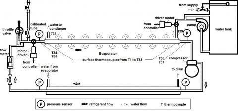
2.1 The primary test rig
The primary test rig, Figure 1, was implemented according to Naas [8] and it consists mainly of the following components;
The Compressor is of type TECUMSEH sealed hermetic reciprocating type of one HP, 220 volts, and 50 Hz.
The Condenser is a heat exchanger which consists of two concentric copper tubes, and have a length of 1700 mm. The inner tube, where the refrigerant flows, has an outer diameter of 9.52 mm,( 3/8 inch), and the inner diameter of 7.72 mm, (2.47/8 inch). The outer tube, where the water flows, has an outer diameter of 19.05 mm,( 3/4 inch), and the inner diameter of 17 mm, (0.68 inches).
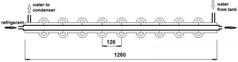
The Main Evaporator, Figure 2, is a heat exchanger which consists of two concentric copper tubes and has a length of 1260 mm. The outer tube, where the water flows, has an outer diameter of 19 mm, and the inner diameter of 17 mm. The outer tube is divided into 10 segments, each segment has an independent inlet and exit terminals. This structure promotes the turbulent mixing activities of the flowing water and accordingly,
enhances the evaporation of the flowing refrigerant. The inner tube, where the refrigerant flows, has an outer diameter of 9.5 mm and an inner diameter of 7.5 mm. The refrigerant mass flow rate and accordingly the Reynolds number could be varied by a valve whose opening is controlled by a stepper motor.
The Pump is QB Series Peripheral 0.25 hp water pump, and it is interfaced to the controller which maintains the water discharge at a fixed rate of 0.74 kg/s.
Figure 1. The primary test rig
Figure 2. The main evaporator
2.2 The measuring and control devices
The signals from thermocouples, pressure sensors, and the flow rate sensors are fed from the microcontroller to a PC program, which calculates the corresponding heat flux, the Reynolds number, and the Nusselt number, Eq. (1-13).
2.3 The experimental procedure
Before beginning, the following procedure is followed;
In every experiment, the following steps were followed;
Table 2. Preparing the Nano-Lubricant
|
Nano-Particles concentration, z |
Z = 0.05 % |
Z = 0.3 % |
Z = 0. 5 % |
Z = 1 % |
|
Lubricant, (gram) |
3 |
18 |
30 |
60 |
|
R134a, (gram) |
596.7 |
580.2 |
567 |
534 |
|
Nano-, (gram) |
0.3 |
1.8 |
3 |
6 |
${{T}_{s,\,av}}\,=\frac{\sum\limits_{1}^{33}{{}}{{T}_{s\,i}}}{33}$ (1)
$T_{si}= T_{top}+T_{bottom}+T_{side}$ (2)
${{T}_{nf,\,av}}\,=(\,{{T}_{in}}\,+{{T}_{out}}\,){{\,}_{nf}}/2$ (3)
According to Nass [8], the volume fraction, the density and the specific heat are calculated as follows;
$100\,\,\varphi \,=\,\,\frac{z{{\rho }_{f}}}{{{\rho }_{np}}\,(1-z)+z{{\rho }_{f}}}$ (4)
${{\rho }_{nf}}=\,\,\varphi \,{{\rho }_{np}}\,+\,(1-\varphi ){{\rho }_{f}}$ (5)
$C{{p}_{nf}}\,=\,\,\frac{\varphi \,{{(\rho \,Cp)}_{np}}\,+(1-\varphi )\,{{(\rho \,Cp)}_{f}}}{{{\rho }_{nf}}}$ (6)
And according to Subramani [10];
$µ_{nf}=µ_f [ 1/(1-φ)^{2.5}]$ (7)
And according to sanukrishna [2];
$k_{nf}/k_f =(k_p+2k_f-2φ(k_f-k_p ))/(k_p+2k_f-φ(k_f-k_p ) )$ (8)
$\overset{*}{\mathop{\text{m}}}\,\,=\,{{(\overset{*}{\mathop{\text{V}}}\,\,\rho )}_{\text{nf}}}$ (9)
$\operatorname{Re}\,=\,\,\frac{4{{\overset{*}{\mathop{m}}\,}_{nf}}}{{{10}^{3}}\pi \,{{d}_{i}}L\,\,{{\mu }_{f}}\,}$ (10)
The program estimates an initial water flow rate, $m*_w$ from an intended heat flux according to;
$\overset{*}{\mathop{q}}\,\,{{A}_{s}}=\,{{\overset{*}{\mathop{m}}\,}_{w}}\,{{C}_{w}}({{T}_{iw}}-{{T}_{ow}})$ (11)
${{h}_{\,}}\,=\,\,\frac{{{[\overset{*}{\mathop{m}}\,\,\,Cp\,({{T}_{o}}-{{T}_{i}})]}_{\,nf}}}{\pi \,{{d}_{i}}L\,({{T}_{s,\,av}}-{{T}_{nf,\,av}})}$ (12)
$Nu\,=\,\,\frac{{{10}^{3}}\,h\,{{d}_{i}}}{{{k}_{nf}}}$ (13)
The cycle coefficient of performance;
$C.\,O.\,P\,=\,\,\frac{Cp\,({{T}_{o}}-{{T}_{i}}){{]}_{\,nf,e}}}{Cp\,({{T}_{o}}-{{T}_{i}}){{]}_{\,nf,c}}}$ (14)
The worst relative errors that may occur when measuring the above quantities are illustrated in Appendix A.
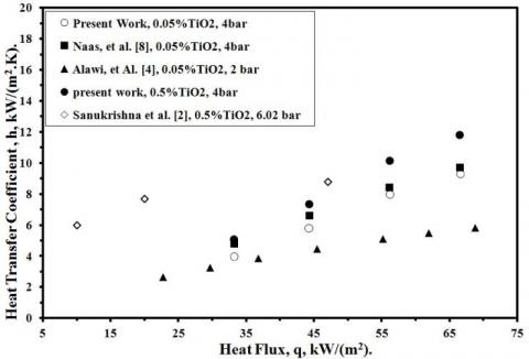
Some of the experimental results of the heat transfer coefficient of the used nano-refrigerant, TiO2/R134a are illustrated in figure 3. The figure also illustrates the results of Naas, [8], Alawi, et al, [4] and Sanukrishna et al. [2] for the same nano- refrigerant but, at different pressure values. It is obvious that all the cases have the same trend of variation but, the results of the present work are more close to those of Naas because both cases have the same conditions of the applied pressure and particle concentration and. As mentioned above, increasing the operating pressure results in an enhancement in the heat transfer coefficient, Cieśliński and Kaczmarczyk [20]. The results of Alawi were obtained under lower pressure than what was applied in the present work. Whereas, the applied pressure in the case of Sanukrishna was higher than that of the present work.
Figure 3. Data from the present work and from Alawi [4], Naas [8] and Sanukrishna [2] at different pressure conditions
3.1 The experimental results
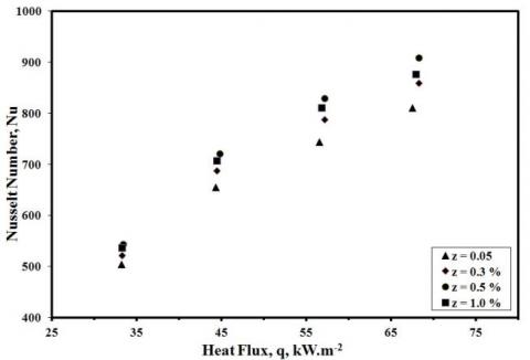
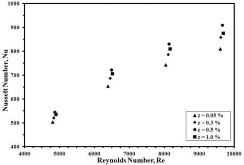
These experiments are executed to investigate the variation of the Nusselt number, with the heat flux and the Reynolds number. Figure 4 illustrates the variation of Nusselt number with the heat flux and Figure 5 illustrates the variation of Nusselt number with the Reynolds number. First observation in Figure 5 is that the position of each data point of the heat flux and the Reynolds number differs slightly with the increase of particles concentration. That is because increasing the concentration leads to an increase in the mass flow rate and accordingly, the Reynolds number slightly increases for the same flow rate. The thermal conductivity and the thermal transport capabilities increase with the concentration too, and this affects the heat flux for the same flow rate. For all studied cases, the Nusselt number increases with the particles concentration until z=0.5% and beyond this value, it starts to decrease again. That may be because, when the particles concentration increases, the mass flow rate increases, equation 4, 5 and 9, and accordingly the mixture thermal conductivity and capacity of carrying more heat increase too. In such conditions, the possibility of increasing the bulk fluid temperature increases. So, the difference in temperature between the fluid and the surface decreases, which helps the heat transfer coefficient to increase, Eq. 12.
The thermal conductivity also increases with the concentration, equation 8, at a lower rate than that of the heat transfer coefficient, and this helps the Nusselt number to increase too equation 13. But, increasing the particles concentration may lead to narrower passages for the particles to move through the fluid and a reduction in the Nano-Particles mobility under the thermophoretic forces and accordingly, its convective heat transfer decreases. So, increasing the Nano-Particle concentration produces two opposing factors; one promotes for the increase in Nusselt number, which is dominant for a Nano-Particles concentration less than 0.5 %, and the other decays it, which starts to be dominant for z>0.5 %.
In Figure 4, the Nusselt number increases with the heat flux, for all values of concentration. That may be because, increasing the heat flux, promotes for a higher refrigerant superheat, which in turn increases the average refrigerant temperature and reduces the temperature difference between the refrigerant and the surface. This leads to an increase in heat transfer coefficient, but a small increase in the refrigerant thermal conductivity, which depends mainly on the temperature, and the majority of the process in the evaporator is a phase change, and accordingly, the Nusselt number increases.
From Figure 5, the Nusselt number increases with the Reynolds number, for all values of concentration. That may be because, increasing the fluid flow rate promotes for a higher possibility of exchanging more thermal energy with the tube surface, which leads to a decrease in the average temperature difference between the surface and fluid, meanwhile, the heat transfer is increased. That may results in a higher heat transfer coefficient with a little change in the thermal conductivity. Consequently, the ratio between the heat transfer and the thermal conductivity increases and accordingly, the Nusselt number increases. The maximum percentage of enhancement in the Nusselt number was 112 % and occurred when increasing the Reynolds number by about 99.7 % of its lowest value.
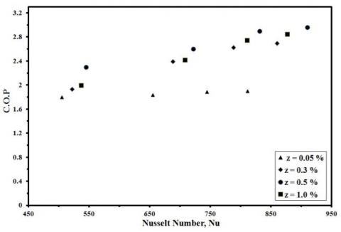
Figure 6 illustrates the variation of C.O.P with heat transfer coefficient. For all Nano-Particle concentration, the C.O.P varies slightly with the Nusselt number, which reflects that, the ratio of the heat transfer rate and the compressor power increase slightly with the Nusselt number. In other words, the compressor power and the cycle losses are almost proportional to the refrigerant mass flow rate. But the relation between the heat transfer rate and the refrigerant mass flow rate is not linear. For the same Nusselt number, the rate of heat transfer increased with the particle concentration with a little increase in the compressor power, so, the COP increased. And again the concentration of Nano-Particles considerably affects the heat transfer, and slightly increases the compressor power, which leads to an increasing COP whenever the particle concentration is lower than 0.5 %. This behavior is reversed when the particle concentration exceeds 0.5 %, where the Nusselt number starts to decrease for the reasons mentioned above.
Figure 4. Variation of Nusselt number with the heat flux
Figure 5. Variation of Nusselt number the reynolds number
Figure 6. Variation of C.O.P with the Nusselt number for different nano-particle concentrations
After trying different formulas to fit the experimental data, one of them could fit the data with minimum deviation, equations 15. This equation relates the Nusselt number to the Nano-Particle concentration, the Reynolds number, and the heat flux. The worst deviation of the calculated Nusselt values from these measured by the correlation was about 5%. Appendix B illustrates samples of the calculated and measured data.
Nu = 0.18 z 0.02 x Re 1.1 x q -0.36(15)
3.2 Controlling the Nusselt number
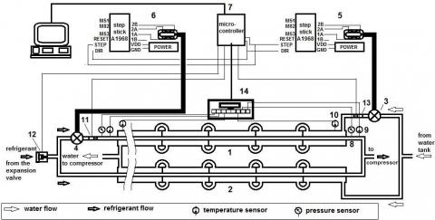
In these experiments, it is required to vary the Nusselt number of the main evaporator with time according to a predetermined behavior. Figure 7 illustrates the preparation of the control experiment. The figure illustrates a secondary evaporator, which is similar to the main evaporator, is installed to share the water and refrigerant flow rates. The two controlled valves are installed in the entrance to the main evaporator; one of them controls the refrigerant flow rate and the other controls the hot water flow rate. The experimental data of the heat flux, Reynolds number and the Nusselt number that is extracted from the experiments, whose Nano-Particles concentration is 0.5 % are fed to the program. According to these data, the controller produces the required variation in the heat flux, the Reynolds number and accordingly, the required Nusselt number. To execute this type of experiments, the preparations and steps from (1 to 5) that are mentioned in 2.2 are followed and then;
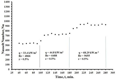
(1) The controller should adjust the system actuators to produce a Reynolds number of about 4866 and a heat flux of 33.4 kW/m2 which correspond to a Nusselt number of about 575. Then, it should maintain the Nusselt number at this value for 60 minutes.
(2) Next, the controller should adjust the Nusselt Number value to be 720 approximately which corresponds to a Reynolds number of 6488 and a heat flux of 44.8 kW/m2. Then, it should maintain the Nusselt number at this value for 80 minutes.
(3) Finally, the controller should adjust the Nusselt Number value to be 910 approximately which corresponds to a Reynolds number of 9655 and a heat flux of 68.3 kW/m2. Then, it should maintain the Nusselt number at this value for 100 minutes.
During the operation, the data of the Nusselt number are monitored every 10 minutes. Figure 8 illustrates the variation of the Nusselt number with time. It is observed that, the Nusselt number value during each of the three time intervals is not stable, that is because, at the beginning of each interval, the controller changes the heat flux and Reynolds number according to the values that are mentioned above, and a PID scheme helps these quantities to approach almost a steady value, and consequently, a required Nusselt value. This scheme keeps guarding the achieved values to maintain them from the random change in the ambient conditions and unpredicted losses. Also, the limited speed, memories, and storage capacity of the used controller did not ensure the proper speed of response to the feedback signals. That is beside the fluctuating nature of the variation in the ambient conditions during the day hours, which is an inherent characteristic of the weather in the city, where these experiments are performed. These random variations may lead to unpredicted losses in the hot water side as well as the refrigerant side of the refrigeration.
1- Main evaporator; 2- secondary evaporator; 3- water control valve; 4- refrigerant control valve; 5- stepper motor+driver, (water valve); 6- stepper motor+driver, (refrigerant valve); 7- microcontroller; 8- refrigerant pressure sensor; 9- refrigerant temperature sensor; 10- water temperature sensor; 11- main evaporator refrigerant flow sensor; 12- total refrigerant flow sensor; 13- main evaporator water flow sensor; 14- thermocouple interface
Figure 7. The control unit installation
Figure 8. The control experiment
An experimental investigation was executed to study the variation of the 'evaporator ' Nusselt number with the heat flux, Reynolds number, at four values of Nano-Particles concentration, (z), in a vapor compression refrigeration system, whose refrigerant is a TiO2/R134a Nano-Fluid. The Nusselt Number increased with the Reynolds number and heat flux in all studied cases. It also increased with the Nano-Particle concentration to the value of 0.5% and beyond this value, a deterioration appeared in its enhancement. The percentage of increase in the Nusselt number achieved a maximum value of 67% when increasing the Reynolds number by about 98% of its lowest value.
Next, the test rig was modified with a secondary evaporator and a control unit which will store the experimental data of the heat flux and the Reynolds number along with the nano-particle concentrations. These data guided the controller to follow a predetermined variation in the Nusselt number and accordingly, to control the cooling behavior.
The experimental results suggested a correlation which expressed the variation of the Nusselt number with both; the Reynolds number and the heat flux at different values of the Nano-Particle concentrations. The present work may be considered as a step to future work, in which, a Nano-Refrigerant system contains a single compressor, that supplies many evaporators situated in different regions in the installation.
Alphabetic
A area m2
cp specific heat W.(kg.K)
di test section inner diameter m
h heat transfer coefficient W/(m2.K)
k thermal conductivity W/(m .K)
l test section length m
m* mass flow rate kg/s
Nu Nusselt number
Q rate of heat transfer W
q* heat per unit surface area W/m2
Re Reynolds number
T temperature K
V volume m3
z mass fraction %
Subscripts
av average.
c condenser
e evaporator
f fluid, (R134a + oil)
i inlet \ inner
np Nano-Particles
nf Nano-Fluid
o outlet
P nano-particle
s surface
w water
Greek symbols
$\delta$ difference
$\phi$ volume fraction
$\mu$ dynamic viscosity Pascal.s
$\rho$ density kg/m3
Abbreviations
C O P coefficient of performance
LCD liquid-crystal display
PID proportional, integral and derivative
POE polyester oil
TiO2 titanium dioxide
Appendices
Appendix A: Error analysis
To estimate the uncertainties of the derived quantities, $\delta$z, $\delta$f and $\delta$h, etc, we first recall the uncertainties of the participating quantities, which are;
Length is measured using a vernier caliper with uncertainty ± 0.02 mm
Temperature: the resolution of the digital indicator is ± 0.1 oC.
The Nano-refrigerant volume flow rate,$\overset{*}{\mathop{\text{V}}}\,$, is measured with an uncertainty of 0.05 L/min
Mass is weighed with the readability of 0.01 gm.
Then, we can estimate the uncertainties in the derived quantities as follows;
$d z=(\frac{\text{ }{{\text{m}}_{\text{np}}}\text{ }\,}{{{\text{m}}_{\text{np}}}+{{\text{m}}_{\text{f}}}})\,\sqrt{{{(\frac{\text{ }\delta \text{ }{{\text{m}}_{\text{np}}}\text{ }\,}{{{\text{m}}_{\text{np}}}})}^{2}}+(\frac{\,\delta \text{ }{{\text{m}}_{\text{np}}}^{2}\,+\,\delta \text{ }{{\text{m}}_{\text{f}}}^{2}\,}{{{\text{(}{{\text{m}}_{\text{np}}}\,+{{\text{m}}_{\text{f}}})}^{2}}})}$ (A.1)
$d f =\,\frac{\text{z }{{\rho }_{\text{f}}}\text{ }\,}{{{\rho }_{\text{np}}}\text{ (1-z)}\,+\text{ z}{{\rho }_{\text{f}}}\text{ }}\sqrt{{{(\frac{\text{ }{{\rho }_{\text{f}}}\text{ }\delta \text{ z }\,}{{{\rho }_{\text{f}}}\text{ }z})}^{2}}+\frac{{{({{\rho }_{\text{np}}}\text{ }\delta \text{ z)}}^{\text{2}}}\text{ }+\text{ }{{({{\rho }_{\text{f}}}\text{ }\delta \text{ z)}}^{\text{2}}}\text{ }\,}{{{({{\rho }_{\text{np}}}\text{ (1-z)}\,+\text{ z}{{\rho }_{\text{f}}}\text{ )}}^{\text{2}}}}}$ (A.2)
$dρ_{nf} =\,\sqrt{{{(\text{ }\delta \,\varphi \,{{\rho }_{\text{np}}}\text{ })}^{2}}+{{(\text{ }\delta \,\varphi \,{{\rho }_{\text{f}}}\text{ })}^{2}}}$ (A.3)
$\,\delta \overset{*}{\mathop{m}}\,\,\,=\,(\,\overset{*}{\mathop{V}}\,\text{ }{{\rho }_{\text{nf}}}\text{) }\sqrt{{{(\frac{\text{ }\delta \text{ }\overset{*}{\mathop{V}}\,\text{ }\,}{\overset{*}{\mathop{V}}\,})}^{2}}+\,{{(\frac{\delta {{\rho }_{\text{nf}}}\text{ }\,}{{{\rho }_{\text{nf}}}})}^{2}}}$ (A.4)
$\delta \,C{{p}_{nf}}=\frac{\,\varphi {{\rho }_{\text{np}}}\,Cp{{\text{ }}_{\text{np}}}\,+\text{(1-}\varphi \text{)}{{\rho }_{f}}\text{ }Cp{{\text{ }}_{\text{f}}}\,}{{{\rho }_{\text{nf}}}}\text{ }\sqrt{\frac{\text{ (}{{\rho }_{\text{np}}}\,Cp{{\text{ }}_{\text{np}}}\,\text{ }\delta \text{ }\varphi {{)}^{2}}+{{\text{(}{{\rho }_{f}}\text{ }Cp{{\text{ }}_{\text{f}}}\,\text{ }\delta \text{ }\varphi )}^{2}}}{\text{ (}\varphi {{\rho }_{\text{np}}}\,Cp{{\text{ }}_{\text{np}}}\,+\text{(1-}\varphi \text{)}{{\rho }_{f}}\text{ }Cp{{\text{ }}_{\text{f}}}\,\text{ }{{\text{)}}^{\text{2}}}}+\,{{(\frac{\text{ }\delta {{\rho }_{\text{nf}}}}{\text{ }{{\rho }_{\text{nf}}}})}^{2}}}$ (A.5)
$\,\delta \,{{\mu }_{nf}}=\,{{\mu }_{\,f}}\text{ (1-}\varphi {{\text{)}}^{\text{2}\text{.5}}}\sqrt{{{(\frac{\text{ }\delta {{\mu }_{\,f}}\text{ }\,}{{{\mu }_{\,f}}})}^{2}}+2.5\,(\frac{\text{ }\delta \varphi \,}{\text{(1-}\varphi ){{\,}^{3.5}}})}$ (A.6)
$\,\delta \,{{k}_{nf}}=\,\sqrt{{{(k\,{{\rho }_{np}})}^{2}}\,[{{(\frac{\delta {{k}_{f}}\,}{{{k}_{f}}\,}\text{)}}^{\text{2}}}\text{ }+{{(\frac{\delta {{\rho }_{f}}\,}{{{\rho }_{f}}\,})}^{2}}]+\,{{[(1-\varphi ){{k}_{f}}]}^{2}}\,[{{(\frac{\delta \varphi \,}{\varphi \,}\text{)}}^{\text{2}}}\text{ }+{{(\frac{\delta {{k}_{f}}\,}{{{k}_{f}}\,}\text{ })}^{2}}]\,\,}$ (A.7)
$\,\delta \operatorname{Re}\,=\,\frac{\overset{*}{\mathop{m}}\,d\,\,}{A\mu }\text{ }\sqrt{{{(\frac{\text{ }\delta \text{ }\overset{*}{\mathop{m}}\,\text{ }\,}{\overset{*}{\mathop{m}}\,})}^{2}}+3\,{{(\frac{\text{ }\delta \,D\text{ }\,}{D})}^{2}}+\,{{(\frac{\text{ }\delta \,\mu \text{ }\,}{\mu })}^{2}}}$ (A.8)
$\,\delta h\,\,=\,\frac{{{[\overset{*}{\mathop{m}}\,\,\,Cp\,({{T}_{o}}-{{T}_{i}})]}_{\,nf}}}{\pi \,{{\text{d}}_{\text{i}}}\text{L }({{T}_{s,av}}-{{T}_{nf,av}})}\text{ }\sqrt{{{(\frac{\text{ }\delta \text{ }\overset{*}{\mathop{m}}\,\text{ }\,}{\overset{*}{\mathop{m}}\,})}^{2}}+{{(\frac{\text{ }\delta \,Cp\text{ }\,}{Cp})}^{2}}+\,{{(\frac{\delta {{T}^{2}}+\delta {{T}^{2}}\text{ }\,}{{{({{T}_{O}}-{{T}_{i}})}^{2}}})}^{2}}+{{(\frac{\text{ }\delta \,{{d}_{i}}\text{ }\,}{{{d}_{i}}})}^{2}}+{{(\frac{\text{ }\delta \,L\text{ }\,}{L})}^{2}}\,+{{(\frac{\delta {{T}^{2}}+\delta {{T}^{2}}\text{ }\,}{{{({{T}_{s,av}}-{{T}_{f,avi}})}^{2}}})}^{2}}}$ (A.9)
$\,\delta \,Nu\,=\,\frac{h\,d}{k}\text{ }\sqrt{{{(\frac{\text{ }\delta \text{ }\overset{*}{\mathop{h}}\,\text{ }\,}{h})}^{2}}+{{(\frac{\text{ }\delta \,d\text{ }\,}{d})}^{2}}+\,{{(\frac{\delta k\text{ }\,}{k})}^{2}}}$ (A.10)
$\delta \,(C.\,O.\,P)\,=\,\,\frac{{{[Cp\,({{T}_{o}}-{{T}_{i}})]}_{\,nf,e}}}{{{[Cp\,({{T}_{o}}-{{T}_{i}})]}_{\,nf,c}}}\,[{{(\frac{2\delta \,Cp\,}{Cp\,})}_{e}}^{2}+\frac{4\,\delta {{T}^{2}}\text{ }\,}{{{({{T}_{O}}-{{T}_{i}})}^{2}}_{c}}\,]$ (A.11)
According to the above formulas, the worst relative errors in the measured quantities are;
Relative error in measuring the weight raTiO2 = 0.0017.
Relative error in measuring the volume fraction = 0.0016.
Relative error in measuring the nano-fluid density = 1.6 e-005.
Relative error in measuring the mass flow rate = 0.027.
Relative error in measuring the nano-fluid specific heat = 2.01 e-5.
Relative error in measuring the heat flux = 0.025.
Relative error in measuring the Nusselt number = 0.0123819.
Relative error in measuring the COP = 0.0294.
Appendix B: Tests of the suggested Correlation
-----------------------------------------------------------
COEFFICIENTS OF EQUATION (15)
0.18 0.02 1.1 -0.36
-----------------------------------------------------------
Correlation Experimental Percentage
-----------------------------------------------------------
512.60 505 1.5
631.09 655 -3.6
743.38 744 -0.08
846.72 811 4.4
539.22 522 3.3
665.51 688 -3.2
780.91 788 -0.8
882.80 860 2.6
549.02 545 0.7
686.88 722 -4.8
794.03 831 -4.4
898.82 910 -1.2
564.08 537 5.0
693.70 708 -2.0
813.17 811 0.2
919.31 877 4.8
[1] Patil MS, Kim SC, Seo JH, Lee MY. (2016). Review of the thermo-physical properties and performance characteristics of a refrigeration system using refrigerant-based nanofluids. Energies 9(1): 22. https://doi.org/10.3390/en9010022
[2] Sanukrishna SS, Ajmal N, Prakash MJ. (2018). Thermophysical and heat transfer characteristics of R134aTiO2 nanorefrigerant: A numerical investigation. 28th International Conference on Low Temperature Physics (LT28) IOP Publishing IOP Conf. Series: Journal of Physics: Conf. Series 969(2018): 012015. https://doi.org/10.1088/1742-6596/969/1/012015
[3] Yang L, Hu YH. (2017). Toward TiO2 Nanofluids—Part 2: Applications and Challenges 12: 446. https://doi.org/10.1186/s11671-017-2185-7
[4] Alawi OA, Mohammed HA, Sidik NAC. (2014). A comprehensive review of fundamentals, preparation, and applications of nano-refrigerants. International Communications in Heat and Mass Transfer 54: 81-95. https://doi.org/10.1016/j.icheatmasstransfer.2014.03.001
[5] Kolekar RD. (2014). An experimental study of the flow boiling of refrigerant-based nanofluids. Dissertation, Phd, The Graduate College of the University of Illinois At Urbana-Champaign.
[6] Ajuka LO, Odunfa MK, Ohunakin OS, Oyewola MO. (2017). Energy and exergy analysis of vapour compression refrigeration system using selected eco-friendly hydrocarbon refrigerants enhanced with TiO2-nanoparticle. International Journal of Engineering & Technology 6(4): 91-97. https://doi.org/10.14419/ijet.v6i4.7099
[7] Yong H, Bi SS, Shi L. (2006). Refrigerator with R134a/TiO2 nanoparticle system, Huagong Xuebao/ Journal of Chemical Industry and Engineering (China) 57: 141-145.
[8] Naas KSM. (2016). Heat transfer enhancement in vapor compression refrigeration system using nano-fluid with R-134a. Thesis, Benha University, Faculty of Engineering, Mechanical Engineering Department.
[9] Javadi FS, Saidur R. (2016). Energetic, economic and environmental impacts of using nanorefrigerant in domestic refrigerators in Malaysia. Energy Conversion and Management 73: 335-339. https://doi.org/10.1016/j.enconman.2013.05.013
[10] Subramani N, Mohan A, Prakash JM. (2013). Performance studies on a vapour compression refrigeration system using nano-lubricant. International Journal of Innovative Research in Science, Engineering and Technology 2(Special Issue 1). Proceedings of International Conference on Energy and Environment-2013 (ICEE 2013) On 12th to 14th December.
[11] Padmanabhan VMV, Palanisamy S. (2012). The use of TiO2 nanoparticles to reduce refrigerator ir-reversibility. Energy Conversion and Management 59: 122-132. https://doi.org/10.1016/j.enconman.2012.03.002
[12] Adelekana DS, Ohunakina OS, Babarindea TO, Odunfaa MK, Leramoa RO, Oyedepoa SO, Badejoa DC. (2017). Experimental performance of LPG refrigerant charges with varied concentration of TiO2 nano-lubricants in a domestic refrigerator. Case Studies in Thermal Engineering 9: 55-61. https://doi.org/10.1016/j.csite.2016.12.002
[13] Dhamneya AK, Rajput SPS, Singh A. (2018). Comparative performance analysis of ice plant test rig with TiO2-R134a nano refrigerant and evaporative cooled condenser. Case Studies in Thermal Engineering 11: 55-61. https://doi.org/10.1016/j.csite.2017.12.004
[14] Bi SS, Guo K, Liu ZG, Wu JT. (2011). Performance of a domestic refrigerator using TiO2-R600a nano-refrigerant as working fluid. Energy Conversion and Management 52(1): 733-737. https://doi.org/10.1016/j.enconman.2010.07.052
[15] Raghavalu KV, Reddy PS, Khan AR, Kumar DV, Prashanth T. (2016). Improvement of COP of vapor compression refrigeration system by using nano-refrigerants. IJSRD || National Conference on Recent Trends & Innovations in Mechanical Engineering || April, pp. 172-175.
[16] Gill J, Singh J, Ohunakin OS, Adelekan DS. (2018). Energy analysis of a domestic refrigerator system with ANN using LPG/TiO2–lubricant as replacement for R134a. Journal of Thermal Analysis and Calorimetry 135(1): 1-14. https://doi.org/10.1007/s10973-018-7327-3.
[17] Ray M, Deb S, Bhaumik S. (2017). Experimental investigation of nucleate pool boiling heat transfer of R134a on TiO2 coated TF surface. Materials Today: Proceedings 4(9): 10002-10009. https://doi.org/10.1016/j.matpr.2017.06.310
[18] Ray M, Bhaumik S. (2018). Nucleate pool boiling heat transfer of hydro-fluorocarbon refrigerant R134a on TiO2 nanoparticle coated copper heating surfaces. Heat Transfer Engineering. https://doi.org/10.1080/01457632 .2018.1450333
[19] Coumaressin T, Palaniradja K. (2014). Performance analysis of a refrigeration system using nano fluid. International Journal of Advanced Mechanical Engineering 4(4): 459-470.
[20] Cieśliński JT, Kaczmarczyk TZ. (2011). The effect of pressure on heat transfer during pool boiling of water-Al2O3 and Water-Cu nanofluids on stainless steel smooth tube. Chemical and Process Engineering 32(4): 321-332. https://doi.org/10.2478/v10176-011-0026-2