Marco Bietresato* | Fabrizio Mazzetto
© 2020 IIETA. This article is published by IIETA and is licensed under the CC BY 4.0 license (http://creativecommons.org/licenses/by/4.0/).
OPEN ACCESS
A problem that is common in agriculture but not very publicized, thanks to the absence of victims, is the rollover of Centre Pivot and Lateral Move irrigation systems. These accidents are due to particularly-strong winds acting on the spans, and they are potentially very destructive for the installations. Also, the restoration phase of the installations requires always an intervention of lifting of the machinery on the field, with a potential further damage to crops (setting) and land (compaction). Given the basic inevitability of the phenomenon, due to atmospheric events, these rollovers could be however limited e.g. by proposing a system design granting a higher stability. Therefore, we have firstly modelled the rollover dynamics of these systems, considering the geometry, the masses, the forces acting on them (wind, gravity), the position of the centre of gravity. Then, thanks to morphometry, we have investigated booms’ stability as a consequence of a proportional or not-proportional alteration of the system sizes, in particular: the upscaling of supports, done by some manufacturers, and the lengthening of spans, often required by customers. Morphometry is a method born in biology, typically used to describe and analyse statistically the shape variations within and among samples of organisms as a result of growth, experimental treatments or evolution. As the idea of evolutionary adaptation is intrinsic in the technical evolution of human-made systems (models, variants) operated by manufacturers, also artificial systems can be studied or improved via the morphometry, as operated here. The output of this study is a physical model of rollover and a sensitivity analysis of a reference configuration for an irrigation boom. Thanks to these analyses, we were able to demonstrate, for example, how a scaling-up of boom supports, respectful of geometric ratios, can increase the system stability despite the elevation of the pressure point of the wind on the frame.
rollover of agricultural equipment, centre pivot and lateral move irrigation systems, morphometry, proportional upscaling / downscaling of a system, sensitivity analysis
1.1 The irrigation systems
An irrigation system is an artificial system used to supply the crops water requirements not satisfied by rainfall [1]. A first classification of these systems can be done considering how the water is distributed on the field, so it is possible to have: gravity-driven (or flood) systems and pressure-driven irrigation systems. All the pressure-driven irrigation systems have one or more pumps, several pipes and a water intake. The different types of irrigation systems can also be classified into fixed, semi-fixed, movable depending on the time-continuity of their positioning on a parcel of land during their lifespan [2, 3]. Another classification concerns the functionality of the irrigation systems, distinguishing them into static or self-propelled systems, depending on whether they have parts that change their position with regard to the area to be irrigated when they are active. Modern self-propelled irrigation systems are driven by hydraulic, thermal or electric motors controlled by a central control-unit. The spread of self-propelled irrigation systems has recently seen a significant increase [3]. The strength point of these systems, which favoured their first diffusion (to give an example of their spreading, in 2002 there were 42,000 pivot systems in Nebraska [4]), is the high water-distribution efficiency obtained with very low water pressures (about 0.70 to 1.05 bar). Other than limiting the energy consumption, the reduced operating pressure avoids the water nebulisation at the sprinklers, which would lead to losses in performance due to the droplets evaporation and the wind-induced drift. Moreover, in these last years, the diffusion of this type of irrigation systems has been further favoured by their possibility of adopting increasingly-sophisticated technologies for the control and the localised management of the irrigation rate [5], e.g.: electro-actuated pressure regulators, remote controls using the GSM/GPRS data networks, guidance systems using the GNSS technology, multi-platform monitoring software programs. Indeed, thanks to the possibility to locate exactly the sprinklers on the ground to be irrigated, these irrigation systems are able to introduce the precision agriculture principles also at the stage of the crops care [6].
This study focuses in particular on Centre Pivot and Lateral Move (or linear move or wheel-move) irrigation systems, which are pressure-driven movable self-propelled wheeled irrigation systems that apply water to pastures or crops, from above the canopy using one or two lines of sprinklers [7]:
Figure 1. (A) first element of a rotating self-propelled irrigation system (“centre-pivot” irrigation system); (B) element of a translating self-propelled irrigation system (or “lateral move” irrigation system)
Centre Pivot and Lateral Move systems have many similitudes:
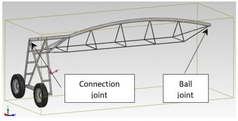
Figure 2. 3D-CAD model of a base element composing a self-propelled irrigation system
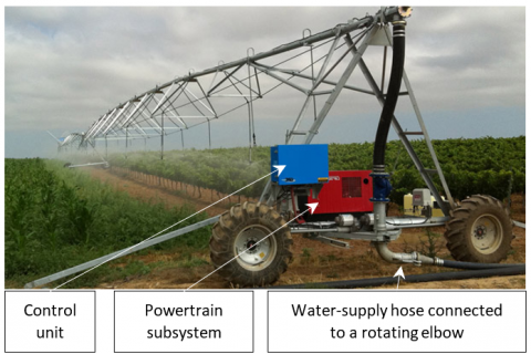
Self-propelled irrigation systems of this type have therefore the following elements [5] (Figure 3):
Figure 3. First motorized support of a lateral move system [5, 8-10]; a typical dimension for the wheels of these systems is 380/85 R24
The limits of use of these wheeled irrigation systems are principally given by the size of the agricultural parcel on which they will operate for at least 20 years after the installation, i.e. the period of time generally needed for an adequate economic amortization of these systems. In Italy, these systems are mainly used in the flat areas of the north, i.e. along the valley of the river Po and in the plains of Veneto and Friuli. In general, such systems are widespread mainly where there are extensive crops (such as: corn and soy) and industrial crops (such as: tomato, sweet corn, potatoes). So, the size of the field parcels, where these irrigation machines are installed in Italy, spans from about 5-6 hectares to more than 80 hectares.
1.2 The risk of rollover of irrigation systems
Even if pivot and lateral move systems are theoretically “movable” (according to the definitions given at the beginning of the previous paragraph), they will be difficultly moved away from the original place of installation, due to their important dimensions and masses. Hence, even when not in operation, these systems are exposed to the inclemency of the weather, with serious risks to be overturned by wind (as documented in Pampa, State of Texas, USA, in 2015 and in other occasions using remote-sensing imagery [12-14]) and, hence, to be damaged in the rollover [11] or to hurt people (e.g. typically the persons that are trying to move their irrigation system below a shelter during a windstorm).
The lateral overturning is a dangerous event in which a system changes its roll angle in a not-controlled way: it undergoes a rotation around an axis approximatively parallel to its longitudinal axis, thus changing its contact points with the ground. Terrestrial systems/vehicles experience overturning when the direction of the resultant of the active forces acting on the centre of gravity (CoG) intercepts the support plane outside of the support polygon (defined by taking the footprints of the system supports as its vertices). This geometrical condition could happen when there is a modification of the direction of the above-cited resultant (e.g., in the case of irrigation systems, when there is a strong wind impacting on the frame) or when the support plane changes locally its inclination (e.g., in the case of self-propelled irrigation systems, due to the harshness of the ground experienced by the system wheels) [15]. In the agricultural engineering field, this phenomenon has been investigated especially with reference to farm tractors [16-20] but also to robots [21]. Indeed, the side-overturning of agricultural machines is a very important problem because it is the principal cause of deaths recorded every year [22-27].
1.3 Aims of this study
In this study:
More specifically, the present study will try to give an answer to the following questions:
2.1 The morphometric approach to the study of natural and artificial systems
Morphometry (or, better, “Geometric morphometry”) is a method used for the statistical analysis of the shapes of objects or living beings belonging to a similitude group [28-32]. It is based on the measurement of some characteristic dimensions obtained from the Cartesian coordinates of some landmark points, previously localized on the objects or living beings under study. The subsequent calculation of the dimensional ratios between these dimensions allows performing comparisons or evidencing similarities and differences among single items or individuals.
The morphometry is applied in many fields of knowledge, from biology to engineering. In particular in biology, this method has many applications in the investigation of variability and evolution of populations of living beings. Indeed, Darwin [33] had demonstrated since 1859 that the shape of an individual is the most evident expression of his genome under the evolutionary thrusts of the environment surrounding a population of individuals. Consequently, Klingenberg [34] uses morphometry to analyse quantitatively the variations in the organismal size and shape of a population. Antonucci et al. [35] study the temporal evolution of species and quantify the differences between isolated populations of individuals of the same species. By doing so, they manage to observe evolutionary convergences/divergences [36].
But, as observed by Hull and Dennett in their respective studies [37, 38], the Darwin’s basic scheme of variation, selection and inheritance can be applied to the evolutionary processes that can be experienced in different domains (“universal” or “generalized” Darwinism applied to evolutionary systems), including also artificial systems. Indeed, it is possible to observe that many artificial systems undergo an evolution (involving also their shape) model after model, exactly as observable for natural systems generation after generation. An initial design of a technical system can evolve according to the principles of differentiation and similitude, for example to satisfy the ever-new requests coming from customers (e.g., new functionalities) and from the marketing department (e.g., product repositioning) [39]. In particular, this can be successfully realized if the modular-design, the parametric-design concepts [40] or other design tools [41] are applied since the very concept of the system, to create an artefact family [42]. For example, in the last 60 years European utilitarian cars has evolved toward a more similar fusiform and compact shape, as emerged by the application of morphometry [43, 44]. Many examples can be found also in the agricultural engineering field: Kutzbach [45] observed the increase of complexity of farm machinery due to the progressive introduction of new/upcoming technical systems; Renius in 1994 [46] tried to figure out a scenario for European tractors based on the trends in tractor design observed till that year, proven effectively to be correct nowadays; Reece [47] studied the shape of farm tractors and its factors of influence, understanding already in 1970 that only a radical change of form could have given a real improvement in the performances; Guzzomi & Rondelli [48] used morphometry to inquiry the energy-absorption capability of the protective structures of 326 modern narrow-track tractors over 16 years; Bietresato et al. [49] analyse 1418 OECD test reports to evidence a substantial invariance of the front-rear masses distribution notwithstanding a constant increase of all dimensions of farm tractors over the last 60-70 years.
In all the above-cited articles, the morphometry proved to be a very effective tool to analyse historical data related to aesthetics and, in general, to the shape of technical systems, evidencing the historical trends of some important/selected characteristics. Furthermore, as many other tools of analysis, it lets a designer capitalize the experiences of the past making them available for the future. So, morphometry can also be used as a real support to the design of a new system or to the study of the evolution of an existing system basically in two ways:
Therefore, in the following paragraphs, a generic self-propelled irrigation system will be firstly analysed by a geometrical point of view, in accordance with morphometry principles: a base element will be isolated and a frame simplification will be operated to recognize the reference shape for the stability condition. After that, following again the morphometry principles, a parametrization of all dimensions will lead to writing a series of equations able to express the stability condition by varying the main dimensions. A particular design solution (i.e., the use of a flexible joint between two adjacent base elements) will be also discussed to understand whether it can effectively be considered a feature really improving the stability of the system (and, hence, an evolution). Then, two scenarios of modifications of the system dimensions, changing or not an important dimensional ratio of the system, will be analysed. Finally, a case study will be presented.
3.1 Rollover stability condition(s) for self-propelled irrigation systems with a flexible joint at the pipe end
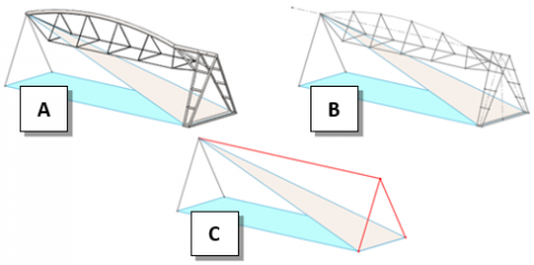
As previously described, these irrigation systems are modular, being composed by the repetition of a base element, and they have a prevailing longitudinal development: the stability condition will be therefore referred to the rollover in the transverse direction of a single base element. The first step is the recognition of the reference frame for the base element (in red in Figure 4), in order to evidence the support points and plot the support polygon, to be intended as the geometrical figure linking all the frame supports. Indeed, the stability condition of a spatial structure or of a vehicle on a ground is verified when there is an intersection of the direction of the resultant of the active forces with the support polygon. As reported in [11]: "the spans are equipped with flexible joints at the ends, allowing the pipeline side-to-side, up and down and rotational movements with no stress on the pipeline". As a consequence, the reference frame is a non-regular tetrahedron, each base element has three support points (two on the ground through the wheels and one on the base element to which it is connected, in correspondence to the ball joint or Cardan joint used to connect two subsequent base elements) and the support polygon is a triangle (Figures 4 and 5, grey polygon). If the connection of each base element with the other base elements were rigid, the support polygon would be a rectangle having as vertices: the centres of the wheels of the base element under study and the centres of the wheels of the base element connected at the span extremity (Figure 4, light blue polygon).
Figure 4. (A to C) process of frame simplification and shape recognition for the base element of a self-propelled irrigation system
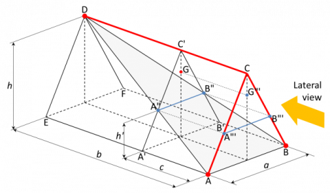
Figure 5. Reference frame for the base element of a self-propelled irrigation system (in red) with in evidence: the support polygon ABD (in grey), the reference shape for the tower ABC, the segment of stability A″B″
If the CoG of the base element (ABCD in Figure 5) is named G, using the schematization proposed in Figure 4, it is possible to evidence the transversal plane A'B'C' containing G (parallel to the vertical plane passing through the tower supports ABC), evidencing the intersection A″B″ of A'B'C' with the support triangle ABD. This segment is very important in the inquired case: as the active forces acting on a base structure are all perpendicular to its longitudinal axis, as well as the resultant of these forces (see the following paragraph for details), the stability condition can be proven when the resulting force direction intersects that segment (which can be rightfully called: “stability segment”). The length a′ and the height h′ of the stability segment are given by the following equations (refer to Figures 5 and 6 for the significance of symbols):
$a^{\prime}=a \cdot \frac{b-c}{b} ; h^{\prime}=h \cdot \frac{c}{b}$ (1)
Figure 6. Reference frame for the base element of a self-propelled irrigation system (in red) seen from a direction parallel to the longitudinal axis of the structure
Therefore, in this case only, the general spatial stability condition can be enunciated as a two-dimensional stability condition (refer to Figure 6, where the system is seen according to the orange arrow of Figure 5, i.e. from a direction parallel to the longitudinal axis of the system): the structure is stable if the direction r of the resultant of the active forces, applied to the base element CoG (in green in Figure 6), has an inclination angle α with the vertical direction lower than the stability angle αL1 (referred to the extremity of the stability segment A”B” ≡ A”’B”’). This is equivalent to observe the sign of the algebraic sum of the moments of each active force on the structure, calculated with A”≡ A”’ as pole: the structure is stable when this sum is positive (i.e., if the resulting moment would cause a clockwise rotation around the pole).
If hG is lower than h, the same condition can be further simplified by referring to the base segment AB ≡ A’B’ of the tower, hence without the need to calculate the position of the extremal points of the segment A”B” ≡ A”’B”’: the structure is stable if the direction r of the resultant of the active forces has an inclination angle α with the vertical direction lower than the stability angle αL2 (< αL1). This is equivalent to observe the sign of algebraic sum of the moments of each active force of the structure, calculated with A ≡ A’ as pole (simplified two-dimensional stability condition). By doing so, thanks to the condition αL2 < αL1,, a higher safety standard will be ensured.
3.2 Discussion upon the influence of the flexible joint height on the rollover stability condition
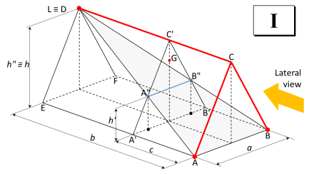
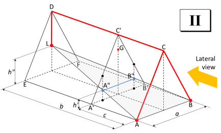
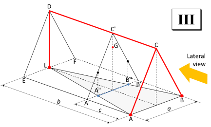
The situation presented above is now generalized, discussing the influence, on the rollover stability condition, of the height h″ at which the connection point L with another base element is located, being equal the position of the base element CoG and of all the other geometric dimensions. Graphically, the situation is represented in the following Figure 7, which shows two limit cases (I and III) and a generic intermediate case (II). As can be seen from the 2D diagram of Figure 7, a variation of the height h″ of the connection point L has a direct influence on the height h′ of the stability segment A″B″ (in blue in Figure 7; as visible, this segment undergoes a progressive elevation if the connection point L is raised) and on the limit angle αL for the lateral overturning, but a′ remains constant:
$h^{\prime}=h^{\prime \prime} \cdot \frac{c}{b}$ (2)
$\alpha_{L}=\arctan \frac{a^{\prime}}{2 \cdot\left(h_{G}-h^{\prime}\right)}$ (3)
Figure 7. (I, II, III at the top) Reference frame for the base element of a self-propelled irrigation system (in red) with the connection point L at three different heights; (at the bottom) view of the same reference frame from a direction parallel to the longitudinal axis of the structure
The displayed situation is also useful for comparing the lateral stability of a system with three supports on staggered support planes (such as the generic case proposed here) and a system with four supports, representative instead of a condition of rigid connection between adjacent elements (i.e., the situation presented in Figure 4). Specifically, the stability of these two systems is the same when the points G, A″ and A′ are aligned (i.e., the limit line rL from G and A″ passes also through A′), hence when the following condition is verified:
$\frac{h^{\prime \prime}}{h_{G}}=1 \Leftrightarrow \frac{h^{\prime}}{h_{G}}=\frac{c}{b}$ (4)
If $h^{\prime \prime} / h_{G}>1 \Leftrightarrow h^{\prime} / h_{G}>c / b$, the stability of a 3-support system is higher than the stability of a 4-support system; this can happen if the connection point L is very high or if the base element CoG is very low: this means that the technical choice of connecting two adjacent base elements through a flexible joint at the end of the main pipe (the highest component of a base element) is fully justified by the safety of the system. In the same way, also the positioning of all power subsystems (i.e., the drivetrain) as low as possible in the tower frame is justified.
3.3 Forces acting on a base element as a function of its dimensions and graphical discussion of possible design alternatives
Systems, such as the one under examination, operate always on lands that are horizontal and flat or, possibly, made flat after an appropriate levelling. Any worsening of the stability conditions due to the ground characteristics, i.e. due to the presence of a slope or of harshness, is therefore excluded and, consequently, the tower frame is supposed in a perfectly-horizontal starting position (Figure 8).
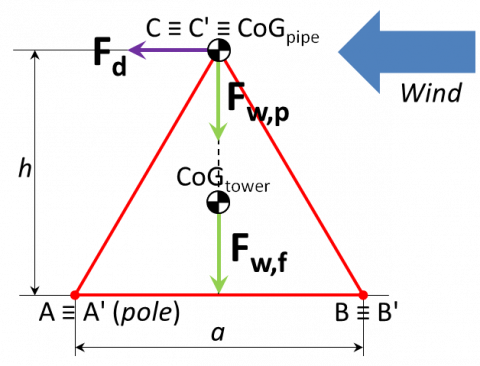
Figure 8. Base element frame of a self-propelled irrigation system viewed from a direction parallel to its longitudinal axis; in evidence the active forces acting on it
Excluding the constraint reactions, the following (active) forces act on a base element (Figure 8):
$F_{d}=c_{d} \cdot \rho_{a i r} \cdot A \cdot \frac{v^{2}}{2}=c_{d} \cdot \rho_{a i r} \cdot\left(D_{p} \cdot \ell_{p}\right) \cdot \frac{v^{2}}{2}$ (5)
$F_{w, f}=g \cdot \overbrace{\rho_{l, f} \cdot \ell_{t o t, f}}^{m_{f}}=g \cdot \rho_{l, f} \cdot(a+2 \cdot \sqrt{h^{2}+\frac{a^{2}}{4}}) \cdot n=g \cdot \rho_{l, f} \cdot a \cdot(1+2 \cdot \sqrt{\frac{h^{2}}{a^{2}}+\frac{1}{4}}) \cdot n=\rho_{l, f}\left(s_{b}\right) \cdot a \cdot k_{f}\left(\frac{h}{a}\right)$ (6)
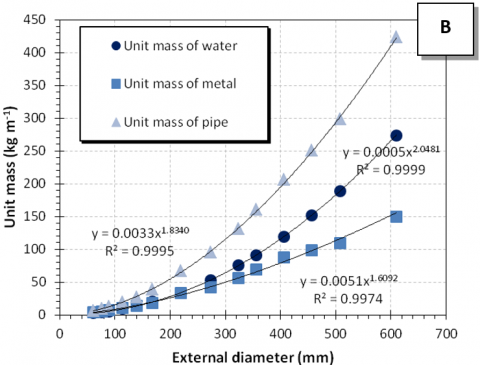
$F_{w, p}=g \cdot m_{p}=g \cdot \rho_{l, p}\left(D_{p}\right) \cdot l_{p}$ (7)
Figure 9. Parametrization of the unit mass of metal pipes (A: welded; B: not welded) starting from the mass of metal and of the water contained in them
Looking from a lateral point of view, a base element is stable if the sum ∑Mi of all the moments of the active forces (net moment) is positive or, in other words, if the sum of the stabilizing moments ∑Mstab (due to the weight forces of the tower and the pipe) is greater than the overturning moment Movert (due to the drag force), all calculated with reference to A ≡ A′ as pole (according to the simplified 2-D stability condition):
$\sum M_{i}>0 \Leftrightarrow \sum M_{s t a b}>M_{\text {overt}} \Leftrightarrow\left(F_{w, f}+F_{w, p}\right) \cdot \frac{a}{2}>F_{d} \cdot h$$\Rightarrow F_{w, f}\left(s_{b}, a, \frac{h}{a}\right)+F_{w, p}\left(D_{p}, \ell_{p}\right)>F_{d}\left(D_{p}, \ell_{p}, v\right) \cdot 2 \cdot \frac{h}{a}$ (8)
Starting from the last inequality, the following two scenarios can be studied.
(I: variation of a) Chosen the pipe dimensions (basically dependent on the hydraulic features of the system) and the beam section (for small variations of the irrigation system size, it can be kept the same, considering an over-dimensioning of the structure aimed at the standardization of components), if the dimensional ratio h/a is fixed (e.g., 0.866 for an equilateral triangle), when scaling up and down the dimensions of the tower, the only term changing is the Fw,f (proportional to a). This means that if a is greater than a threshold value alim that is a function of the wind speed (it is a size limit), the system is stable and increasing the design value of a (→ different design choice: scaling up) gives a more stable system.
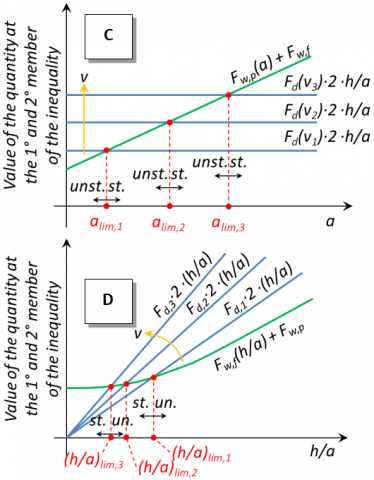
In the same way, for an already-built system (a is set), when the wind speed v rises (→ change in operating conditions), the threshold value alim rises proportionally with v2 and, if alim overcomes the current value of a, the system overturns (Figure 10); analogously, starting from the same inequality, it is possible to calculate the maximum value of wind speed vlim that can be undergone by the system:
$a_{l i m}(v)=\frac{F_{d}\left(v^{2}\right)-2 \cdot \frac{h}{a} \cdot F_{w p}}{\rho_{l, f} \cdot k_{f}}$ (9)
$v_{l i m}=\sqrt{2 \cdot \frac{\rho_{l, f} \cdot k_{f} \cdot a+2 \cdot \frac{h}{a} \cdot F_{w p}}{c_{D} \cdot \rho_{a i r} \cdot\left(D_{p} \cdot \ell_{p}\right)}}$
(II: variation of h/a) Chosen the pipe dimensions (basically dependent on the hydraulic features of the system) and the bean section (for small variations of the irrigation system size, it can be kept the same, considering an over-dimensioning of the structure aimed at the standardization of components), set the base width a, when altering the dimensional ratio h/a (→ different design choice) to raise or lower the pipe height (in accordance with the customer/crop needs), the terms that change are Fw,f and the quantity that multiplies Fd in the second member of the inequality. As there exists a threshold value for h/a, i.e. (h/a)lim, which makes equal the two members of the inequality, the effect of an increase of the ratio h/a is to decrease the value of this threshold, making the structure reach an instability condition (Figure 10). In the same way, also an increase of the wind speed (→ change in operating conditions) has the effect of decreasing the value of the threshold (h/a)lim (Figure 10): the instability occurs when (h/a)lim becomes lower than h/a.
Figure 10. Effect of an increase of a (A) or of h/a (B) on the system stability; interpretation of an increase of v on the system size limit alim (C) or shape limit (h/a)lim (D); the system is stable when the green line (1st member of the inequality (8)) is above the blue line (2nd member of (8))
3.4 A case study: The exceptional downburst recorded at Rosolina Mare (province of Rovigo, Italy) on 10th August 2017
The equations presented here will be now applied to study the possibilities for a real lateral move irrigation system to resist a storm that really happened at “Po di Tramontana” (45° 4' 3.753" N, 12° 15' 39.633" E), c/o Rosolina (province of Rovigo, Italy), on 10th August 2017. As visible from Figure 11, the meteorological station at Po di Tramontana recorded an increasing wind speed starting from 12:00 of that day due to a so-called “downburst” phenomenon, reaching a peak value of 16.1 and 21.1 m s-1 at 2 and 10 m height from the ground, respectively, at 14:30. Unfortunately, the maximum values (gust wind value) are not available due to a technical problem that occurred at the same meteorological station. The storm, which happened in that place, has been chosen as case-study because it caused many damages to many man-made infrastructures, as documented by the television news and the newspaper articles published the following day.
Figure 11. Average wind speed during the day of 10th August 2017 (source: ARPAV)
Thanks to the historical data put at our disposal by the Regional Agency for the Environmental Protection – Region of Veneto, Italy (ARPAV), it has been possible to plot the return period curves for that place. The reference period for these data is 01/01/1992 - 28/05/2019, corresponding to 10 009 days. The following Figure 12 will show:
As can be calculated from the interpolating equations reported in Figure 12, the return periods corresponding to the peak values of the average speed at 2 and 10 m height recorded on 10th August 2017 are respectively 2337 and 1691 years, thus giving an idea of the exceptionality of the occurred event for that place. The maximum wind speeds (gust wind speeds) in correspondence to those return periods are respectively 31.9 m s-1 (114.8 km h-1) and 38.6 m s-1 (138.8 km h-1), which can be used as a good indication for the gust wind speeds to substitute for the real values unfortunately not recorded by the meteorological station.
Finally, as the considered irrigation systems have the main pipe at a height of 4 or 5 m from the ground [5, 8-10] (Table 1), an exponential interpolating function has been calculated starting from the data at 2 and 10 m height, with the aim of giving an estimation of the wind speed at 4 or 5 m. For the average wind speed the passage points for calculating the equation coefficients are (16.1 m s-1, 2 m) and (21.1 m s-1, 10 m), for the gust wind speed the passage points are (31.9 m s-1, 2 m) and (38.6 m s-1, 10 m). A linear interpolation between the same two points, although simpler, would have underestimated the wind speed between 2 and 10 m height, as it would have completely neglected the curvature of the speed profile that is usually present in these cases. Therefore, it follows:
$h=k_{1} \cdot e^{k_{2} \cdot v} \Rightarrow k_{1}=0.0112 ; k_{2}=0.3219$ (10)
for the average wind speed
$h=k_{1} \cdot e^{k_{2} \cdot v} \Rightarrow k_{1}=9.411 \cdot 10^{-4} ; k_{2}=0.2402$ (11)
for the gust wind speed
Figure 12. (A) absolute maximum wind speed (gust wind speed) above 16 and 20 m s-1 at 2 and 10 m and (B) maximum average wind speed measured at 2 and 10 m from the ground with the relative return periods
Thanks to these equations, we obtain for the two heights of respectively 4 and 5 m from the ground:
The first quantity to calculate is the Reynolds number for four typical dimensions of the main pipe [5, 8-10] (Table 2), to verify the flow-regime characteristics (ρa is the density of the air in kg m-3; v is the velocity of the air/wind with respect to the pipe in m s-1; Dp is the pipe diameter in m; μa is the dynamic viscosity of the air in Pa·s or N·s m-2 or kg (m·s)-1):
$\mathrm{Re}=\rho_{a} \cdot v \cdot D_{p} / \mu_{a}$ (12)
The results in Table 2 indicate a fully-developed turbulent flow, close to the laminar-to-turbulent transition for the boundary layer (for the gust speed), and, for both the speeds (average, gust), very far from the vortex-shedding condition (very dangerous for the structure for the periodicity, the entity and the direction: when it is upwards it acts as a lift force and can aggravate the stability). In this case it is possible to state that the only aerodynamic force on the pipe is the drag force (parallel to the wind speed; see Figure 8).
Table 1. Main dimensions for the two considered sizes for the tower
|
Quantity |
Unit |
Value |
|
|
Low profile |
High profile |
||
|
Base element width (a) |
m |
2.70 |
5.15 |
|
Base element height (h) |
m |
3.47 |
4.47 |
|
Frame dimensional ratio (h/a) |
- |
1.29 |
0.87 |
|
Wheels diameter (ref. measure 380/85 R24) |
m |
1.06 |
1.06 |
|
Height of the pipe centre from the ground (htot) |
m |
4.00 |
5.00 |
|
Angle at the top vertex |
° |
42.5 |
59.9 |
|
Angle at the base vertexes |
° |
68.8 |
60.1 |
Table 2. Reynolds number and drag coefficient for different diameters of the water pipe
|
Quantity |
Unit |
Value |
||||
|
Pipe nominal diameter |
in |
6 5/8 |
8 |
8 5/8 |
10 |
|
|
Linear mass (metal) |
kg m-1 |
22.0 |
29.8 |
33.6 |
42.4 |
|
|
Linear mass (water) |
kg m-1 |
21.1 |
31.1 |
36.3 |
48.8 |
|
|
Ave. wind speed |
Reynolds nr. at 4 m |
- |
210,754 |
254,554 |
274,503 |
317,176 |
|
Reynolds nr. at 5 m |
- |
218,718 |
264,173 |
284,876 |
329,161 |
|
|
Drag coeff. (cD) |
- |
1.0 |
1.0 |
1.0 |
1.0 |
|
|
Gust wind speed |
Reynolds nr. at 4 m |
- |
401,425 |
484,852 |
522,849 |
604,128 |
|
Reynolds nr. at 5 m |
- |
412,159 |
497,816 |
536,830 |
620,282 |
|
|
Drag coeff. (cD) |
- |
0.6 |
0.3 |
0.3 |
0.3 |
|
Then, we calculated the total weight force of the pipe (empty) and of the tower, the drag force on the pipe (five lengths) and the respective moments of these forces with reference to a vertex of the tower frame (simplified two-dimensional stability condition), in this case A ≡ A′ according to Figure 8. The net moments on the system (∑Mi in equation 8), calculated as the difference between the stabilizing moments and the overturning moment, are reported in Table 3.
As visible, all the numbers reported in Table 3 are positive, meaning that the studied systems are not overturned by constant winds having the indicated values. Indeed, for these systems, the maximum value of wind speed vlim are 42.4 and 54.1 m s-1, respectively, for the low- and high-profile system (Dp 6 5/8″, Lp 66 m), both higher than the estimated gust wind speed. This is consistent with a statement by Guyer & Moritz [4] about centre pivot irrigators: most of them are designed to withstand 130 km h-1 (36.1 m s-1) winds when empty of water. However, overturning may anyway occur due to regularly-pulsating gusts and to the consequent swinging movement than can be triggered by them (not investigated here).
Finally, it is possible to observe that the low-profile system (htot = 4 m) has net moments always smaller than the high-profile system (htot = 5 m), meaning that the low-profile system has a shape potentially more critical. This is due to the h/a ratio of the low-profile that is smaller than that of the high-profile system, thus prevailing as effect on the stability, notwithstanding that the high-profile has a greater overturning moment due to its higher position of the pipe.
Table 3. Net moments (in N m) acting on a base element of a self-propelled irrigation system
|
htot |
v |
Lp |
Pipe nominal diameters |
|||
|
m |
m s-1 |
m |
6 5/8″ |
8″ |
8 5/8″ |
10″ |
|
4.00 (low prof.) |
18.26 (ave.) |
43 |
14,074 |
17,463 |
19,173 |
23,164 |
|
49 |
15,050 |
18,887 |
20,824 |
25,344 |
||
|
55 |
16,023 |
20,310 |
22,473 |
27,521 |
||
|
61 |
17,002 |
21,739 |
24,130 |
29,709 |
||
|
66 |
17,967 |
23,149 |
25,764 |
31,867 |
||
|
34.78 (gust) |
43 |
7,871 |
16,900 |
18,566 |
22,463 |
|
|
49 |
8,024 |
18,250 |
20,137 |
24,550 |
||
|
55 |
8,177 |
19,598 |
21,705 |
26,634 |
||
|
61 |
8,331 |
20,953 |
23,282 |
28,729 |
||
|
66 |
8,482 |
22,289 |
24,837 |
30,795 |
||
|
5.00 (high prof.) |
18.95 (ave.) |
43 |
34,660 |
41,694 |
45,215 |
53,382 |
|
49 |
36,885 |
44,850 |
48,839 |
58,089 |
||
|
55 |
39,105 |
48,001 |
52,456 |
62,787 |
||
|
61 |
41,337 |
51,169 |
56,092 |
67,510 |
||
|
66 |
43,538 |
54,293 |
59,678 |
72,167 |
||
|
35.71 (gust) |
43 |
26,393 |
41,117 |
44,593 |
52,664 |
|
|
49 |
27,521 |
44,197 |
48,134 |
57,275 |
||
|
55 |
28,647 |
47,272 |
51,669 |
61,877 |
||
|
61 |
29,779 |
50,363 |
55,222 |
66,505 |
||
|
66 |
30,895 |
53,410 |
58,726 |
71,067 |
||
A generic self-propelled irrigation system has been successfully analysed by a geometrical point of view, thanks to morphometry. The performed parametrization of all dimensions of the reference frame for this system allows writing several equations able to express the stability condition by varying the dimensions and the features. Specifically, a flexible joint at the end of a span to connect an adjacent base element resulted in raising the stability of the system. This situation falls within a particular geometric condition and its validity limit has been calculated. Then, the same stability condition allows understanding that, in the design of such a system, when scaling up the dimensions of the tower without altering the dimensional ratio h/a, there is an increase in the system stability. Vice versa, an increase of h/a causes a significant decrease of the stability. These evidences have been illustrated theoretically and using a case study in which a real irrigation system (with: 2 tower sizes, 4 pipe diameters, 5 span lengths) faces an exceptional downburst recorded in northern Italy.
The authors wish to thank Dr Marco Martello, Italian professional agronomist and expert in irrigation systems, for the precious explanations concerning the operation of this type of agricultural equipment. The authors deserve also to thanks Dr Marco Monai, head of the Meteorological Centre of ARPAV – Regional Agency for the Environmental Protection – Veneto, Dr Alberto Bonini Baraldi, head of the Agrometeorological Operative Unit of the same Agency, and his collaborator Mr Marco Dianin, for having put at the authors’ disposal the meteorological data used in the exposed case-study.
[1] Utah State University. Utah Vegetable Production and Pest Management Guide - Corn Irrigation. n.d. http://vegetableguide.usu.edu/production/sweet-corn-production/irrigation, accessed on June 6, 2019.
[2] Zema, D.A. Corso di Idraulica Agraria ed Impianti Irrigui - Lezione n. 12: Impianti irrigui per aspersione. Univ Degli Stud Mediterr Di Reggio Calabr 2011:75. https://www.unirc.it/documentazione/materiale_didattico/598_2012_314_14983.pdf, accessed on June 6, 2019.
[3] Comiti, F. (2009). Agricultural Hydrology and Drainage Management - Introduction to Irrigation 2009:45.
[4] Guyer, J.L., Moritz, M.L. (2002). On issues of tornado damage assessment and f-scale assignment in agricultural areas 2002.
[5] Valmont Industries Inc. Valley Product Catalog 2018:28.
[6] Omary, M., Camp, C.R., Sadler, E.J. (1997). Center pivot irrigation system modification to provide variable water application depths. Appl Eng Agric, 13: 235-9. https://doi.org/10.13031/2013.21604
[7] Agriculture Victoria - Irrigation Survey and Designers Group. Centre Pivot and Lateral Move Systems. n.d. http://agriculture.vic.gov.au/agriculture/farm-management/soil-and-water/irrigation/centre-pivot-and-lateral-move-systems, accessed on June 6, 2019.
[8] Valmont Industries Inc. Valley Linears 2018:2.
[9] Valmont Industries Inc. Valley Structures 2018:4.
[10] Valmont Industries Inc. Valley Drive Train 2018:8.
[11] Safa, M., Birendra, K. (2015). Damage reduction methods of centre pivot irrigation systems in windstorms. IRES 6th Int. Conf., Melbourne, Australia: 2015, pp. 144-8.
[12] Womble, J.A., Wood, R.L., Mohammadi, M.E. (2018). Multi-scale remote sensing of tornado effects. Front Built Environ, 4: 66. https://doi.org/10.3389/fbuil.2018.00066
[13] Womble, J.A., Wood, R.L., Smith, D.A., Louden, E.I., Mohammadi, M.E., Leitch, K.R. (2016). Reality capture for tornado damage to structures. Struct Eng - J Struct Eng Assoc Texas 2016. https://doi.org/10.1061/9780784480427.012
[14] Womble, J.A., Wood, R.L., Smith, D.A., Louden, E.I., Mohammadi, M.E. (2017). Reality capture for tornado damage to structures. Struct. Congr. 2017, Reston, VA: American Society of Civil Engineers, pp. 134-44. https://doi.org/10.1061/9780784480427.012
[15] Ahmadi, I. (2011). Dynamics of tractor lateral overturn on slopes under the influence of position disturbances (model development). J Terramechanics, 48: 339-46. https://doi.org/10.1016/j.jterra.2011.07.001
[16] Chisholm, C.J. (1979). The effect of parameter variation on tractor overturning and impact behaviour. Journal of Agricultural Engineering Research, 24(4): 417-40. https://doi.org/10.1016/0021-8634(79)90081-7
[17] Bietresato, M., Carabin, G., Vidoni, R., Mazzetto, F., Gasparetto, A. (2015). A parametric approach for evaluating the stability of agricultural tractors using implements during side-slope activities. Contemporary Engineering Sciences, 8(28): 1289-130. https://doi.org/10.12988/ces.2015.56185
[18] Yisa, M.G., Terao, H., Noguchi, N., Kubota, M. (1998). Stability criteria for tractor-implement operation on slopes. Journal of Terramechanics, 35(1): 1-19. https://doi.org/10.1016/S0022-4898(98)00008-1
[19] Bietresato, M., Mazzetto, F. (2019). Definition of the layout for a new facility to test the static and dynamic stability of agricultural vehicles operating on sloping grounds. Appl. Sci., 9(19): 4135. https://doi.org/10.3390/app9194135
[20] Bietresato, M., Mazzetto, F. (2018). Increasing the safety of agricultural machinery operating on sloping grounds by performing static and dynamic tests of stability on a new-concept facility. International Journal of Safety and Security Engineering, 8(1): 77-89. https://doi.org/10.2495/SAFE-V8-N1-77-89
[21] Vidoni, R., Bietresato, M., Gasparetto, A., Mazzetto, F. (2015). Evaluation and stability comparison of different vehicle configurations for robotic agricultural operations on side-slopes. Biosystems Engineering, 129: 197-211. https://doi.org/10.1016/j.biosystemseng.2014.10.003
[22] INAIL. (2015). Report annuale sugli infortuni mortali e con feriti gravi verificatisi nel 2014 nel settore agricolo e forestale. https://www.inail.it/cs/internet/docs/ucm_184750.pdf, accessed on June 6, 2019.
[23] Rossato, M., Maritan, F. Morti in agricoltura: l’emergenza cresciuta negli ultimi tre anni. n.d. https://www.vegaengineering.com/servizi/105/morti_in_agricoltura:_l’emergenza_cresciuta_negli_ultimi_tre_anni.html, accessed on June 6, 2019.
[24] National Safety Council - Research and Safety Management Solutions Group. (2017). Injury facts. Chicago, Illinois, USA.
[25] Goldenhar, L.M., Schulte, P.A. (1996). Methodological issues for intervention research in occupational health and safety. American Journal of Industrial Medicine, 29(4): 289-94. https://doi.org/10.1002/(SICI)1097-0274(199604)29:4<289::AID-AJIM2>3.0.CO;2-K
[26] Yoder, A.M., Murphy, D.J. (2000). Evaluation of the Farm and Agricultural Injury Classification Code and follow-up questionnaire. J Agric Saf Health, 6(1): 71-80. https://doi.org/10.13031/2013.2913
[27] Váliková, V., Rédl, J., Antl, J. (2013). Analysis of accidents rate of agricultural off-road vehicles. J. Cent Eur Agric, 14(4): 1303-16. https://doi.org/10.5513/JCEA01/14.4.1348
[28] James Rohlf, F., Marcus, L.F. (1993). A revolution morphometrics. Trends in Ecology & Evolution, 8(40: 129-32. https://doi.org/10.1016/0169-5347(93)90024-J
[29] Lawing, A.M., Polly, P.D. (2010). Geometric morphometrics: Recent applications to the study of evolution and development. Journal of Zoolgy, 280(1): 1-7. https://doi.org/10.1111/j.1469-7998.2009.00620.x
[30] Zelditch, M.L., Swiderski, D.L., Sheets, H.D. (2012). Introduction. Geometric Morphometrics for Biologists, 1-20. https://doi.org/10.1016/B978-0-12-386903-6.00001-0
[31] Mitteroecker, P., Gunz, P. (2009). Advances in Geometric morphometrics. Evol Biol, 36: 235-47. https://doi.org/10.1007/s11692-009-9055-x
[32] Costa, C., Antonucci, F., Pallottino, F., Aguzzi, J., Sun, D.W., Menesatti, P. (2011). Shape analysis of agricultural products: A review of recent research advances and potential application to computer vision. Food Bioprocess Technol, 4: 673-92. https://doi.org/10.1007/s11947-011-0556-0
[33] Darwin, C. (1859). On the Origin of Species by Means of Natural Selection. London: John Murray.
[34] Klingenberg, C.P. (2002). Morphometrics and the role of the phenotype in studies of the evolution of developmental mechanisms. Gene, 287(1-2): 3-10. https://doi.org/10.1016/S0378-1119(01)00867-8
[35] Antonucci, F., Boglione, C., Cerasari, V., Caccia, E., Costa, C. (2012). External shape analyses in Atherina boyeri (Risso, 1810) from different environments. Italian Journal of Zoology, 79(1): 60-8. https://doi.org/10.1080/11250003.2011.595431
[36] Antonucci, F., Costa, C., Aguzzi, J., Cataudella, S. (2009). Ecomorphology of morpho-functional relationships in the family of sparidae: A quantitative statistic approach. Journal of Morphology, 270(7): 843-55. https://doi.org/10.1002/jmor.10725
[37] Hull, D.L. (1998). Science as a process: An evolutionary account of the social and conceptual development of science. Chicago and London: The University of Chicago Press.
[38] Dennett, D.C. (1995). Darwin’s Dangerous Idea. Simon & Schuster.
[39] Gautschi, D.A., Sabavala, D.J. (1995). The world that changed the machines: A marketing perspective on the early evolution of automobiles and telephony. Technol Soc, 17: 55-84. https://doi.org/10.1016/0160-791X(94)00026-A
[40] Li, J.S., Chen, L.H., Li, L. (2010). Parametric design of tractor configuration using API based on CATIA. Key Engineering Materials, 455: 411-6. https://doi.org/10.4028/www.scientific.net/KEM.455.411
[41] Chandrasegaran, S.K., Ramani, K., Sriram, R.D., Horváth, I., Bernard, A., Harik, R.F., Gao, W. (2013). The evolution, challenges, and future of knowledge representation in product design systems. Computer-Aided Design, 45(2): 204-28. https://doi.org/10.1016/j.cad.2012.08.006
[42] Guzzomi, A.L., Maraldi, M., Molari, P.G. (2012). A historical review of the modulus concept and its relevance to mechanical engineering design today. Mechanism and Machine Theory, 50: 1-14. https://doi.org/10.1016/j.mechmachtheory.2011.11.016
[43] Costa, C., Aguzzi, J. (2015). Temporal shape changes and future trends in European automotive design. Machines, 3(3): 256-67. https://doi.org/10.3390/machines3030256
[44] Grimson, W., Murphy, M. (2009). An evolutionary perspective on engineering design. In: Christensen, S., Delahousse, B., Meganck M, editor. Eng. Context, Aarhus: Academica, pp. 263-76.
[45] Kutzbach, H.D. (2000). Trends in power and machinery. Journal of Agricultural Engineering Research, 76(3): 237-47. https://doi.org/10.1006/jaer.2000.0574
[46] Renius, K.T. (1994). Trends in tractor design with particular reference to Europe. Journal of Agricultural Engineering Research, 57(1): 3-22. https://doi.org/10.1006/jaer.1994.1002
[47] Reece, A.R. (1970). The shape of the farm tractor. Proc Inst Mech Eng, 184: 125-32. https://doi.org/10.1243/PIME_CONF_1969_184_501_02
[48] Guzzomi, A.L., Rondelli, V. (2013). Narrow-track wheeled agricultural tractor parameter variation. J Agric Saf Health, 19: 237-60. https://doi.org/10.13031/jash.19.10249
[49] Bietresato, M., Bisaglia, C., Merola, M., Brambilla, M., Cutini, M., Mazzetto, F. (2017). An application of morphometry to artificial systems: The evolutionary study of farm tractors. Chemical Engineering Transactions, 58: 145-150. https://doi.org/10.3303/CET1758025