OPEN ACCESS
The residential sector has been achieved in the last years more and more importance in the total energy consumption scenario by stimulating the research for solutions to promote energy efficiency and to raise awareness on energy consumption by end user.
The profile of an end-users energy consumption assumes a central role in finding solutions to reduce energy demand and increase the efficiency in the production of the same energy.
European regulations impose an obligation on Member States to provide annually data on energy consumption of households for end use and energy product. Data will be provided for Italy basing on data collected by ISTAT Survey on energy consumption in the residential sector, appropriately processed by ENEA and ISTAT.
In this paper it is presented a methodology that allowed to define a series of dwelling types, representative of the entire national sample, as a function of building, family and environmental characteristics. These dwellings, through the application of a dynamic simulation model, allowed the generation of monthly energy consumption profiles (for heating, cooling and domestic heat water) for each cluster of dwelling types and the evaluation of the energy consumption distribution of the residential sector for end use and energy product.
Energy consumption, Residential sector, Dwelling types, Energy efficiency, Energy demand.
The European and national policies, aimed at containing the energy product consumption and at promoting the diffusion of renewable sources, have stimulated the search for ways to reduce the energy demand and to boost the efficiency in energy production. In particular, for the residential sector, the knowledge of the consumption habits of the families is of vital importance for achieving the goals set by the various European directives, as well as for raising awareness on energy consumption and for stimulating rational behaviors on energy use by end-users.
The regulation (EC) No 1099/2008 of the European Parliament and of the Council of 22 October 2008 on energy statistics, and the amending Commission Regulation (EU) No 431/2014 of 24 April 2014 on energy statistics, as regards the implementation of annual statistics on energy consumption in households, impose an obligation on Member States to provide annual data on energy consumption of households for final destination and energy source. In this framework, ISTAT in collaboration with ENEA and MiSE (Italian Ministry of Economic Development) carried out the survey on households energy consumption [1, 2], as part of the Italian National Statistics Plan. The survey was conducted in 2013 for the first time in Italy, on a representative sample of 20,000 households at regional level and made it possible to obtain information on characteristics, consumption habits, types of plant and energy costs of Italian households, specified by energy product (primary energy sources and energy carriers) and end-use (heating, cooling, domestic hot water, cooking, lighting and electrical equipment).
This paper describes the methodology used to estimate the energy consumption for heating and the creation of monthly load profiles for residential dwellings. For the sake of simplicity we have chosen to present the results for the Veneto Region and heating systems fueled by natural gas; the calculation method remains the same for other energy products and for the entire Italian national territory.
Furthermore, this methodology will be used in the activity ENEA-ISTAT to estimate the energy consumption of households for the years between two replications of the ISTAT survey, starting from the ISTAT 2016 survey that will be used to deliver the first data to Eurostat.
The presented methodology is based on the processing of the provided statistical data from the ISTAT 2013 survey on households energy consumption, and on the identification of dwelling-type classes representative of the entire Italian residential building stock.
The information provided by the ISTAT 2013 survey and used for the methodology are mainly:
The classification of the dwellings was chosen as a function of:
Table 1 summarizes the 20 identified dwelling-type classes (DTC).
Table 1. Dwelling-type classes
|
Before 1950 |
1950-1969 |
1970-1989 |
From 1990 |
|
|
Single fam. House |
DTC1 |
DTC6 |
DTC11 |
DTC16 |
|
Multi-fam. House |
DTC2 |
DTC7 |
DTC12 |
DTC17 |
|
Ground fl. apt. |
DTC3 |
DTC8 |
DTC13 |
DTC18 |
|
Middle fl. apt. |
DTC4 |
DTC9 |
DTC14 |
DTC19 |
|
Top fl. apt. |
DTC5 |
DTC10 |
DTC15 |
DTC20 |
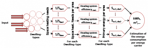
The evaluation of the energy product consumption for heating has been carried out in different stages, as exemplified in Figure 1:
The decision to estimate the thermal energy demand for all the dwelling-types by means of a dynamic simulation of the dwelling, and then calculate the energy product consumption by multiplying the heating demand calculated in continuous mode by the reduction factor for intermittent heating and by the average total efficiency of the heating system was related to the information provided by survey about the type and the characteristics of the heating systems. Clearly, the information provided by the survey can not have a level of detail sufficient to estimate a management profile of the heating systems, which is instead essential to perform a dynamic simulation of the building-plant system.
Since the energy performances of buildings are strongly influenced by climatic conditions, the same dwelling-type was simulated in each climate zone. For each climatic zone in which the country is divided, the input weather data (temperature, radiation and humidity) adopted for the simulations were those of the chief town whose degree days are “barycentric” with respect to the degree days interval of the climatic zone.
Each dwelling-type class is characterized by thermo-physical and dimensional parameters, determined on the basis of both the information gathered from the ISTAT survey results, appropriately processed, and the input data required by the simulation model. Below, the main properties that define each dwelling-type class, are listed and described.
Figure 1. Methodology scheme, for space heating and for a single energy product
Table 2. Thermal transmittance of the opaque envelope by period of build [kW/m2K]
|
Before 1950 |
1950-1969 |
1970-1989 |
From 1990 |
|
|
Walls |
1.093 |
1.065 |
0.675 |
0.456 |
|
Floor |
0.781 |
0.781 |
0.850 |
0.442 |
|
Roof |
1.376 |
1.376 |
0.777 |
0.441 |
Table 3. Thermal trasmittance of the trasparent envelope by period of build and type of dwelling [kW/m2K]
|
Before 1950 |
1950-1969 |
1970-1989 |
From 1990 |
|
|
S. F. House |
3.320 |
3.490 |
3.280 |
2.450 |
|
Multi-fam. House |
3.010 |
3.230 |
2.950 |
2.400 |
|
Apartments |
3.240 |
3.530 |
3.400 |
2.560 |
Table 4. Dwelling-types' heated floor surfaces [m2].
|
Before 1950 |
1950-1969 |
1970-1989 |
From 1990 |
|
|
S. F. House |
121.5 |
115.0 |
119.9 |
130.3 |
|
Multi-f. House |
122.0 |
103.7 |
115.9 |
122.6 |
|
Gr. Fl. Apt. |
86.3 |
92.4 |
82.1 |
83.1 |
|
Mid. Fl. Apt. |
90.8 |
83.6 |
89.1 |
92.8 |
|
Top Fl. Apt |
98.5 |
89.6 |
93.4 |
90.8 |
Table 5. Dwelling walls’ main exposures and consequent simulations.
|
S1 |
S2 |
S3 |
S4 |
S5 |
S6 |
S7 |
S8 |
S9 |
S10 |
|
|
SFH |
all |
- |
- |
- |
- |
- |
- |
- |
- |
- |
|
MFH |
N+S |
E+W |
N+E+S |
- |
- |
- |
- |
- |
- |
- |
|
GFApt |
N |
E |
S |
W |
N+S |
E+W |
N+E |
N+W |
E+S |
S+W |
|
MFApt |
N |
E |
S |
W |
N+S |
E+W |
N+E |
N+W |
E+S |
S+W |
|
TFApt |
N |
E |
S |
W |
N+S |
E+W |
N+E |
N+W |
E+S |
S+W |
|
S1 |
S2 |
S3 |
S4 |
S5 |
S6 |
S7 |
S8 |
S9 |
S10 |
|
|
SFH |
100.0% |
- |
- |
- |
- |
- |
- |
- |
- |
- |
|
MFH |
44.1% |
23.9% |
32.0% |
- |
- |
- |
- |
- |
- |
- |
|
GFApt |
14.2% |
11.7% |
12.6% |
4.9% |
10.5% |
10.8% |
7.6% |
7.6% |
12.4% |
7.9% |
|
MFApt |
14.2% |
11.7% |
12.6% |
4.9% |
10.5% |
10.8% |
7.6% |
7.6% |
12.4% |
7.9% |
|
TFApt |
14.2% |
11.7% |
12.6% |
4.9% |
10.5% |
10.8% |
7.6% |
7.6% |
12.4% |
7.9% |
Since the aim of the work is the determination of both the energy consumption and the thermal load profiles, we chose to use a dynamic simulation model, made by the University of Catania, based on the equivalent resistance-capacitance model proposed in the European standard EN ISO 13790 [4].
Dynamic models for the evaluation of energy consumption in buildings are developed taking into account the variability of both the external climatic conditions of the internal loads. In general, the calculation of the heat load in summer is done with dynamic methods that take into account the thermal capacity and the thermal transients of the buildings.
The European standard EN ISO 13790 proposes an electro-thermal dynamic model simplified with five thermal conductance and a heat capacity, called 5R1C, shown in Figure 2.
Figure 2. 5R1C Model Scheme
The nodes in the model scheme represent the ventilation ($\theta$sup), the outdoor air ($\theta$e), the envelope mass ($\theta$m), the envelope indoor surface ($\theta$s) and the indoor air ($\theta$air) temperatures. The heat transfer coefficients are: the ventilation heat transfer coefficient (Hve), the transmission heat transfer coefficient for windows (Htr,w), the emissive transmission heat transfer coefficient for the opaque envelope towards the envelope mass (Htr,em), the conductive transmission heat transfer coefficient for the opaque envelope towards the envelope indoor surface (Htr,ms), the coupling conductance between the envelope indoor surface and the indoor air (Htr,is). The heat flows are: heat flow rate from internal and solar sources towards the envelope mass ($\Phi$m), heat flow rate from internal and solar sources towards the envelope indoor surface ($\Phi$st), heat flow rate from internal sources towards indoor air ($\Phi$ia), heating or cooling needs ($\Phi$HC,nd).
The EN ISO 13790 standard defines uniquely the heat transfer coefficients and proposes a mode of solution refers to the monthly average daily conditions and monthly average daily time conditions.
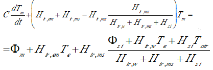
The direct solution, set the temperature and the thermal conductance, allow the calculation of the net flux exchanged, $\Phi$HC,nd, under changing climatic conditions. This solution involves the solution of a differential equation related to the heat balance to $\Phi$m node:
For the net flow we have:
The recursive solution based on Heun method is:
where:
The calculation thus prepared is sufficient and can be quickly implemented on Excel spreadsheet.
The input data required for the model are:
An important feature of the method is the ability to customize the input vectors as a function of weather data, the real profiles for plants and internal gains.
As output, the model provides for each day (representative of the month) a time profile of the latent load, the total load required, the attenuation coefficient, the indoor air temperature and the inner surface of the walls.
The consumption of primary energy from the thermal energy demand is determined according to the following parameters:
The aH,red coefficient takes into account that the plants do not run for all day, the solar and inner gains and the building time constant and are calculated according to the formula proposed in the UNI TS 11300-1 / 2014 [5]:
$a_{H, r e d}=1-b_{H, r e d}\left(\tau_{H, O} / \tau\right) \gamma_{H}\left(1-f_{H, h r}\right)$
The overall performance of thermal plants is calculated as the product of the efficiencies of the subsystems in which is divided, namely the generation, distribution, control and emission.
The efficiency of each subsystem is determined as a weighted average for the plant surface of each type of dwelling inferred from the survey responses, to which a value as indicated in the UNI TS 11300-2 / 2014 [6] was assigned.
The efficiency of the generation subsystem is dependent on the primary source used, while other subsystems are independent. In the case of single or portable heating systems, it was assigned to each type a single overall efficiency.
The types of considered subsystems, are:
• emission: radiators, fan coils and radiant panels;
• control: on-off and thermostatic valves;
• distribution: before and after 1990 with different efficiency values for single and multi-family house, ground floor autonomous apartments, middle and top floor autonomous apartments, last and centralized apartments.
For the generation subsystem supplied by natural gas, it was considered the boiler for centralized and autonomous systems and stoves for those individuals.
Table 7 shows the values of the overall efficiency calculated:
Table 7. Global efficiency of natural gas heating systems, for each dwelling-type class [-]
|
Before 1950 |
1950-1969 |
1970-1989 |
From 1990 |
|
|
S. F. House |
0.767 |
0.765 |
0.767 |
0.768 |
|
Multi-f. House |
0.766 |
0.767 |
0.769 |
0.761 |
|
Gr. Fl. Apt. |
0.794 |
0.788 |
0.792 |
0.771 |
|
Mid. Fl. Apt. |
0.788 |
0.795 |
0.797 |
0.773 |
|
Top Fl. Apt |
- |
0.794 |
0.798 |
0.785 |
The first result, which is also the most important for the many activities in which it can be used, is the classification of the whole Italian residential housing stock in 20 classes of dwelling-types, determined as previously described.
6.1 Thermal load
For each dwelling-type, the profiles of the indoor air temperature, of the thermal energy demand (assuming a continuous heating mode) and of the thermal load (that is the dwelling energy demand with a power profile for a total number of hours equal to the maximum allowed), were obtained.
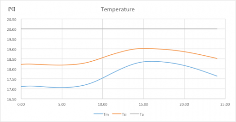
Figure 3, Figure 4 and Figure 5 show an example of the available hourly profiles for the dwelling-type class “top floor apartment”, period of build “before 1950”, in the case of controlled mechanical ventilation.
Figure 3. Indoor temperature hourly profile, continuous heating mode [°C]
Figure 4. Heating demand hourly profile of the average day for each month, continuous heating mode [kW]
Figure 5. Thermal load hourly profile of the average day for each month, intermittent heating mode [kW]
Figure 5 clearly shows how the presence of a power profile highlights a different distribution of the thermal output required by the heating system, providing much more detailed information closer to a real trend.
Figure 6. Monthly heating consumption profile [MWh]
In Figure 6 an example of a monthly consumption of thermal energy for heating profile is plotted: it is referred to a single simulation run of the 34 possible for each period of build and for each climatic zone.
6.2 Energy product consumption
Starting from the results of the 34 simulations performed for each period of build (Table 5), it is possible to obtain the thermal energy consumption of each dwelling-type, as the average weighted on the table of weights (Table 6) multiplied by its corresponding reduction factor for intermittent heating, aH,red (Table 8).
Table 8. Reduction factor for intermittent heating (aH,red) corresponding to each simulation, period of build “before 1950”, climatic zone E [-]
|
S1 |
S2 |
S3 |
S4 |
S5 |
S6 |
S7 |
S8 |
S9 |
S10 |
|
|
SFH |
0.70 |
- |
- |
- |
- |
- |
- |
- |
- |
- |
|
MFH |
0.83 |
0.81 |
0.82 |
- |
- |
- |
- |
- |
- |
- |
|
GFApt |
0.80 |
0.74 |
0.77 |
0.78 |
0.77 |
0.73 |
0.75 |
0.77 |
0.73 |
0.75 |
|
MFApt |
0.71 |
0.62 |
0.66 |
0.67 |
0.72 |
0.68 |
0.70 |
0.73 |
0.67 |
0.70 |
|
TFApt |
0.73 |
0.64 |
0.68 |
0.69 |
0.70 |
0.66 |
0.68 |
0.71 |
0.66 |
0.69 |
Since four periods of build have been identified, for each climatic zone 136 simulations are performed, and their results, weighted on Table 6 and multiplied by their corresponding reduction factors for intermittent heating, allow the calculation of the thermal energy consumption of the 20 identified dwelling-types, as shown in Table 9.
Table 9. Heating consumption for each dwelling-type, climatic zone E [kWhy]
|
Before 1950 |
1950-1969 |
1970-1989 |
From 1990 |
|
|
S. F. House |
19342 |
18232 |
17957 |
18500 |
|
Multi-f. House |
24138 |
21245 |
22979 |
23325 |
|
Gr. Fl. Apt. |
9947 |
11287 |
9802 |
9704 |
|
Mid. Fl. Apt. |
5832 |
5678 |
5966 |
6018 |
|
Top Fl. Apt |
11154 |
9669 |
10774 |
10174 |
Dividing the heating consumption table of the dwelling-types (Table 9) by the table of the dwelling-types' heated floor surfaces (Table 4), the heating consumption per area for each dwelling-type class, for the considered climatic zone, is obtained (Table 10).
Table10. Heating consumption per area for each dwelling-type class, climatic zone E [kWh/m2y].
|
Before 1950 |
1950-1969 |
1970-1989 |
From 1990 |
|
|
S. F. House |
159.20 |
158.54 |
149.77 |
141.99 |
|
Multi-f. House |
197.85 |
204.88 |
198.27 |
190.26 |
|
Gr. Fl. Apt. |
115.27 |
122.16 |
119.39 |
116.78 |
|
Mid. Fl. Apt. |
64.24 |
67.93 |
66.96 |
64.86 |
|
Top Fl. Apt |
113.24 |
107.92 |
115.35 |
112.05 |
The procedure described above is then applied for all climatic zones, and a table similar to Table 10 is obtained for each climatic zone.
For each dwelling-type class, is then possible to calculate the weight of each climatic zone by considering the share of floor surface of the class, falling in each zone: in the case of the Veneto Region, for instance, the single family house class is distributed between zone E (91.5 % of the heated floor surface) and zone F (8.5 % of the heated floor surface).
This distribution is then summarized for each climatic zone, as shown in Table 11 for the climatic zone E.
Table 11. % of floor surfaces of the building-type classes falling in the climatic zone E [-]
|
Before 1950 |
1950-1969 |
1970-1989 |
From 1990 |
|
|
S. F. House |
91.5% |
95.6% |
94.7% |
96.6% |
|
Multi-f. House |
94.6% |
93.4% |
95.6% |
97.2% |
|
Gr. Fl. Apt. |
100.0% |
97.2% |
94.5% |
94.3% |
|
Mid. Fl. Apt. |
96.6% |
95.6% |
98.6% |
100.0% |
|
Top Fl. Apt |
100.0% |
95.9% |
76.4% |
75.8% |
Weighting the simulation results of each climatic zone by the percentage of floor falling in the zone itself, the heating consumption per area for each dwelling-type class is calculated. The results for the Veneto Region are summarized in Table 12.
Table12. Heating consumption per area for each dwelling-type class [kWh/m2y]
|
Before 1950 |
1950-1969 |
1970-1989 |
From 1990 |
|
|
S. F. House |
145.69 |
151.58 |
141.69 |
137.22 |
|
Multif. House |
187.27 |
191.28 |
189.62 |
184.93 |
|
Gr. Fl. Apt. |
115.27 |
118.75 |
112.82 |
110.14 |
|
Mid. Fl. Apt. |
62.03 |
64.92 |
66.01 |
64.86 |
|
Top Fl. Apt |
113.24 |
103.47 |
88.18 |
84.99 |
Multiplying the heating consumption per area by the total area of the dwellings, that use a specific energy product for heating (in the present example: natural gas), that fall in each dwelling-type class (Table 13) and dividing by the respective system’s global efficiency (Table 7), it is possible to assess the total energy product consumption for heating of each dwelling-type class for the specific energy product, as shown in Table 14.
Table 13. Total floor surface of each dwelling-type class, using Natural gas as energy product for heating [m2]
|
Before 1950 |
1950-1969 |
1970-1989 |
From 1990 |
|
|
S. F. House |
5135 |
7785 |
11520 |
5665 |
|
Multi-f. House |
1915 |
4950 |
6370 |
7865 |
|
Gr. Fl. Apt. |
3340 |
7330 |
7375 |
3960 |
|
Mid. Fl. Apt. |
720 |
3135 |
3400 |
2500 |
|
Top Fl. Apt |
0 |
225 |
525 |
690 |
The sum of the elements of Table 14, reporting the total annual consumption of the dwelling-type classes for the considered energy product provides the overall annual energy product consumption for heating of the residential building stock for the considered energy product which, in the case of the Veneto Region and of natural gas, is approx. 15,014 MWh.
Table 14. Total annual energy product consumption for heating of each dwelling-type class, natural gas [MWhy]
|
Before 1950 |
1950-1969 |
1970-1989 |
From 1990 |
|
|
S. F. House |
975.3 |
1542.9 |
2129.3 |
1011.5 |
|
Multi-f. House |
468.3 |
1234.0 |
1570.6 |
1910.9 |
|
Gr. Fl. Apt. |
484.9 |
1105.2 |
1050.0 |
565.4 |
|
Mid. Fl. Apt. |
56.7 |
255.9 |
281.5 |
209.8 |
|
Top Fl. Apt |
0.00 |
29.31 |
58.03 |
74.69 |
The project activity is still in progress. The present step, in progress, is the comparison between the consumption data calculated with the presented methodology and those estimated by the ISTAT survey, the final results of the comparison will be published later.
The above presented methodology has enabled, by means of processing the data on energy consumption of Italian families provided by the ISTAT survey and with the aid of a dynamic simulation model, the realization of a tool able to estimate the energy consumption and to create the thermal load profiles of the representative dwellings of the Italian residential sector.
In particular the methodology allowed to group the entire national sample in 20 cluster of type dwellings, as a function of building (dimensions, equipment, energy characteristics, etc.), family (number of occupants, consumption habits, etc.) and environmental (region, climatic zone, etc.) characteristics.
The methodology is able to estimate energy consumptions distinguished for end use (heating, cooling and domestic hot water) and energy product.
The aim of the work is to increase knowledge of consumer habits of end user to outline a real scenery of the buildings consumption useful to address the choice of the most efficient technological solutions and to provide guidance on the policy actions of support for the dissemination of the most promising technologies.
[1] Istat, (2014, Dec. 15). “I consumi energetici delle famiglie”, Statistiche Report, (In Italian). [Online]. Available: http://www.istat.it/it/archivio/142173.
[2] P. Ungaro, I. Bertini, (2014), “I modelli per la stima dei consumi energetici per finalità d'uso e fonte”. [Online]. Available: http://www.istat.it/it/archivio/141193.
[3] Abaco delle strutture costituenti l'involucro opaco degli edifici - Parametri termo fisici, UNI/TR 11552:2014 Standard, 2014.
[4] Energy performance of buildings - Calculation of energy use for space heating and cooling, EN ISO 13790:2008 Standard, 2008.
[5] Prestazioni energetiche degli edifici. Parte 1: Determinazione del fabbisogno di energia termica dell’edificio per la climatizzazione estiva ed invernale. UNI/TS 11300-1:2014.
[6] Prestazioni energetiche degli edifici. Parte 2: Determinazione del fabbisogno di energia primaria e dei rendimenti per la climatizzazione invernale, per la produzione di acqua calda sanitaria, per la ventilazione e per l'illuminazione in edifici non residenziali. UNI/TS 11300-2:2014.