
Vladimir Konchin* | Irina Vornacheva | Dmitrii Zhilyakov
© 2026 The authors. This article is published by IIETA and is licensed under the CC BY 4.0 license (http://creativecommons.org/licenses/by/4.0/).
OPEN ACCESS
Hardware stability requirements depend on the radar-processing metric they must protect. This study formulates a performance-to-error framework and illustrates it with normalized signal models, without measured component data. The cases comprised a linear-frequency-modulated (LFM) pulse with a time-bandwidth product of 64, Barker-13 compression, a two-pulse moving-target-indication canceller, and an ideal 32-element broadside array. For independent square-law pulse decisions, a 3-out-of-4 rule with a packet false-alarm probability of 10⁻⁶ and a detection-probability decrease from 0.90 to 0.85 allowed a 0.332 dB signal-to-noise-ratio (SNR) loss. The corresponding deterministic chirp-rate-error boundary was 1.83%. Under independent zero-mean Gaussian phase errors, the other boundaries were 10.59° per-chip root-mean-square (RMS) phase error for mean Barker-13 peak sidelobe ratio (PSLR) degradation, 1.81° aggregate differential inter-pulse RMS phase error for mean clutter residual, and 19.77° element RMS phase error for mean array gain. These quantities have different definitions and are not interchangeable component specifications. Equal-share source values and a specified correlated-source example illustrate covariance arithmetic. The results identify the governing metric in each model; practical hardware allocation still requires source sensitivities, measured covariance, and joint nonlinear verification.
active phased array, hardware stability, moving-target indication, pulse compression, radar detection, uncertainty propagation
Pulse compression, coherent integration, moving-target indication (MTI), and digital beamforming depend on waveform and channel coherence. Classical radar detection theory relates detection probability to statistical assumptions about the signal and noise [1]. In hardware, errors arise in frequency synthesis, modulation, amplification, conversion, sampling, and array calibration. A component specification must therefore relate to the processing metric it is intended to protect.
Prior work already links particular hardware errors to radar performance. Siddiq et al. [2] derived source phase-noise limits for frequency-modulated continuous-wave (FMCW) radar and examined decorrelation in coherent mixing. Tschapek et al. [3] separated systematic phase distortion from stochastic phase noise and retained its spectral structure. These studies establish that phase-noise sensitivity depends on the signal model and processing operation; a single integrated phase-error value cannot replace that information. For pulse compression, Bharadwaj and Chandrasekar [4] examined phase-noise effects on sidelobes. Torres et al. [5] explicitly connected waveform design to high-level weather-radar requirements, while enhanced matched filtering [6] addressed sidelobe suppression. Thus, requirement-driven design and phase-error sensitivity are established subjects.
Related studies provide more specific links between hardware instability and the processed signal. Thurn et al. [7] related the source phase-noise profile and range correlation to FMCW ranging uncertainty. Siddiq et al. [8] modeled the contribution of sampling-clock jitter to the phase noise of sampled homodyne signals. Levy et al. [9] examined coherent integration loss under nonstationary phase noise, while Birkenhauer et al. [10] described over-the-air measurement of radar phase-noise spectra. These results show why source spectra, timing, and the receiver architecture must be specified before aggregate signal-error limits can be assigned to hardware.
Spatial processing imposes additional constraints. Geiß et al. [11] related array calibration errors to image distortions and bounded their effects. Beacon-based calibration [12] provides measured channel corrections, whereas auxiliary-array selection [13] concerns adaptive sidelobe cancellation. Studies [12, 13] establish relevant calibration and cancellation contexts; they do not validate a scalar mean-gain budget or the allocation proposed here. Schmid et al. [14] derived worst-case and statistical beam-pattern deviation bounds for calibration errors and mutual coupling, providing a complementary basis for array tolerance analysis. The present array example evaluates only mean gain under independent element phase errors.
This study organizes these function-specific relations into a common sequence: define a performance limit, select an observable metric, identify an error coordinate, and distribute its variance when a stochastic source model is available. The contribution is a mathematical framework illustrated by normalized cases, rather than a complete radar allocation validated with component records. The aim is to compare governing constraints for linear-frequency-modulated (LFM) chirp-rate mismatch, Barker-13 chip phase error, two-pulse MTI differential phase error, and mean array gain. The numerical examples establish aggregate boundaries and illustrate equal-share covariance arithmetic; they do not identify source-specific hardware sensitivities.
2.1 Performance limits and observable signal metrics
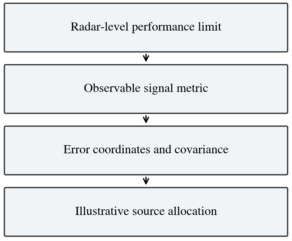
Figure 1 shows the proposed hierarchy. A radar-level limit is converted into a metric at the output of a matched filter, canceller, or beamformer. An error model then relates that metric to waveform or channel perturbations. Hardware allocation additionally requires source sensitivities and covariance. The present examples illustrate the first mappings and a normalized equal-share calculation.
Figure 1. Performance-to-error hierarchy and illustrative allocation
For the j-th radar characteristic, the general mapping is written as
$\Delta C_j=F_j(q), \mathbf{q}=G(\mathbf{x})$ (1)
where, $\Delta C_j$ is the admissible deterioration of a radar-level characteristic, $\mathbf{q}$ is the vector of observable signal metrics, and $\mathbf{x}$ contains deterministic biases and random hardware errors. The first mapping depends on the detection, resolution, cancellation, or beamforming algorithm. The second mapping can be obtained analytically, by circuit-level simulation, or by a controlled numerical perturbation of the signal-processing chain.
For pulse-compression radar, the mismatched-filter output is
$y(\tau ; \mathbf{x})=\int s(t ; \mathbf{x}) s_0^*(t-\tau) \mathrm{d} t$ (2)
where, $s_0(t)$ is the nominal waveform and $s(t ; \mathbf{x})$ is the waveform containing hardware-induced errors. Three complementary metrics are used: the normalized main-peak amplitude $a=|y(0 ; \mathbf{x})| /|y(0 ; \mathbf{0})|$, the peak sidelobe ratio (PSLR) $\delta=$ $\max _{\tau \notin \mathcal{M}}|y(\tau ; \mathbf{x})| /|y(0 ; \mathbf{x})|$, and the relative half-power width increase $\Delta_\tau=$ $\left[\tau_{3 \mathrm{~dB}}(\mathbf{x})-\tau_{3 \mathrm{~dB}}(\mathbf{0})\right] / \tau_{3 \mathrm{~dB}}(\mathbf{0})$. Here, $\mathcal{M}$ denotes the nominal mainlobe interval. For random errors, the mean and variance of each metric are retained rather than only its nominal value.
2.2 Detection-probability mapping
When an $m$-pulse observation uses a "$k$ out of $m$" decision rule, the packet-level probability is related to the single-pulse probability $p$ by
$P(p ; k, m)=\sum_{r=k}^m \frac{m!}{r!(m-r)!} p^r(1-p)^{m-r}$ (3)
Eq. (3) assumes independent pulse decisions with the same single-pulse probability. It was applied separately to detection and false alarms. The detection model used a nonfluctuating target, additive circular complex Gaussian noise, a square-law detector, and a fixed threshold. The normalized detector statistic had two degrees of freedom: a central chi-square distribution under noise alone and a noncentral chi-square distribution with noncentrality 2ν under signal plus noise. Here ν is the single-pulse signal-to-noise-ratio (SNR). The relation is pD = Q₁(√(2ν), √η), where Q₁ is the first-order Marcum Q function and η = −2 ln pF. A fixed receive filter and unchanged noise power were assumed. An amplitude mismatch factor a therefore changed SNR to ν′ = a²ν.
The calculation used a 3-out-of-4 rule, packet false-alarm probability PF = 10⁻⁶, baseline packet detection probability PD,0 = 0.90, and minimum packet detection probability PD,min = 0.85. These are prescribed numerical conditions, not operational requirements for a particular radar. Correlated pulse decisions, target fluctuations, adaptive thresholds, and clutter would require a different probability mapping.
2.3 Criteria for moving-target indication and active arrays
For a two-pulse canceller, let φₙ be the zero-mean residual phase of pulse n and Δφₙ = φₙ − φₙ₋₁ the differential inter-pulse phase error. A stationary unit-amplitude return produces residual power |1 − exp(jΔφₙ)|². If Δφₙ is Gaussian with variance σΔφ2, its mean residual power is
$r_{\mathrm{MTI}}=2\left[1-\exp \left(-\frac{\sigma_{\Delta \phi}^2}{2}\right)\right] \approx \sigma_{\Delta \phi}^2$ (4)
The phase-difference variance is σΔφ2 = Var(φₙ) + Var(φₙ₋₁) − 2 Cov(φₙ, φₙ₋₁). For a stationary process with pulse variance σp2 and lag-one correlation ρ₁, it becomes 2σp2(1 − ρ₁). Independent consecutive pulse errors therefore give σp = σΔφ/√2; this conversion is invalid without the temporal covariance. The residual in Eq. (4) is normalized to the power of one uncancelled pulse. Its −30 dB limit is not an MTI improvement factor normalized to target gain.
For a stationary phase process with one-sided phase-noise power spectral density Sφ(f), σΔφ2 = 4∫₀∞ Sφ(f) sin²(πfTr) df, where Tr is the pulse-repetition interval. The integral must use the phase process at the canceller input, including relevant transfer functions and measurement bandwidth. Thus, an oscillator or clock specification requires Tr and a spectral or temporal model; it cannot be inferred from σΔφ alone.
For an N-element broadside array with equal amplitudes and independent zero-mean Gaussian element phase errors of standard deviation σa, the mean normalized coherent power gain is
$g=\frac{1}{N}+\left(1-\frac{1}{N}\right) \exp \left(-\sigma_a^2\right)$ (5)
where g = E{|N⁻¹∑ exp(jφℓ)|²}, φℓ is the phase error of element ℓ. Eq. (5) concerns this mean alone. Beam-pointing displacement, sidelobe level, and the probability of an individual gain loss were not evaluated. Table 1 distinguishes the quantities actually calculated from error classes that would require additional models.
Table 1. Evaluated quantities and scope of the numerical cases
|
Case |
Evaluated Coordinate and Metric |
|
Linear-frequency-modulated (LFM) |
Prescribed chirp-rate mismatch; detection-derived peak loss and half-power width |
|
Barker-13 |
Independent per-chip Gaussian phase error; mean peak loss and mean peak sidelobe ratio (PSLR) |
|
Two-pulse moving-target indication (MTI) |
Gaussian differential phase error; mean residual power |
|
32-element array |
Independent element Gaussian phase error; mean coherent power gain |
2.4 Covariance propagation and allocation
Let $z_i$ be a selected signal metric and let $x_r$ represent the error generated by the $r$-th hardware source. Linearization about the nominal operating point gives
$\Delta z_i \approx \sum_{r=1}^R S_{i r} x_r, \quad S_{i r}=\left.\frac{\partial z_i}{\partial x_r}\right|_{\mathbf{x}=\mathbf{0}}$ (6)
With the sensitivity row vector $\mathbf{S}_i$ and the hardware-error covariance matrix $\boldsymbol{\Sigma}_x$, the metric variance is
$\sigma_{z_i}^2=\mathbf{S}_i \boldsymbol{\Sigma}_x \mathbf{S}_i^{\top}$ (7)
For independent sources, Eq. (7) reduces to $\sigma_{z_i}^2=\sum_r S_{i r}^2 \sigma_{x_r}^2$. If a fraction $\beta_{i r}$ of the allowable variance is assigned to source $r$, with $\beta_{i r} \geq 0$ and $\sum_r \beta_{i r}=1$, its allowable standard deviation is
$\sigma_{x_r, \max }^{(i)}=\frac{\sqrt{\beta_{i r}} \sigma_{z_i, \max }}{\left|S_{i r}\right|}$ (8)
For each source, the overall allowable standard deviation is the minimum of its criterion-specific values in Eq. (8). This construction assumes independent sources and a nonzero sensitivity for the criterion concerned. A zero sensitivity imposes no first-order restriction and requires higher-order examination. Deterministic biases contribute through the signed sum of sensitivity times bias; root-sum-square (RSS) addition is not a worst-case bias rule. Correlated-source allocation requires the complete covariance expression in Eq. (7), not Eq. (8) alone.
Variance is the square of the standard deviation. For zero-mean errors, root-mean-square (RMS) equals standard deviation; a biased error has RMS² = variance + bias². Moreover, peak loss and mean coherent-gain loss are locally even functions of phase or chirp mismatch and can have zero gradient at the nominal point. Eqs. (6)–(8) must not be applied to those losses using a zero first derivative. The illustrative allocations below operate in additive error coordinates; the processing loss is then evaluated with its nonlinear model.
A practical implementation would define each protected limit, measure or simulate source perturbations, estimate sensitivities, construct the source covariance matrix, and solve the applicable allocation constraints. It would then check the full nonlinear chain at the combined errors. This study did not perform those operations with measured hardware records. The equal-share examples in Section 3.4 demonstrate only the specified normalized source model.
2.5 Numerical models and design limits
The calculations used normalized complex baseband signals. The LFM pulse was s₀(t) = exp(jπKt²), −T/2 ≤ t ≤ T/2, with KT² = BT = 64. Here T is the pulse duration, and B is the bandwidth. A uniform grid of Ns= 1,024 points included both endpoints. The perturbed pulse used K(1 + εK), where the prescribed chirp-rate mismatch εK ranged from 0 to 6% in 0.25-percentage-point increments. Discrete linear correlation implemented Eq. (2). The nominal-delay peak was normalized by Ns; half-power crossings were linearly interpolated. Only the chirp rate was perturbed. Start frequency, duration, general sweep nonlinearity, and phase noise were not evaluated in this case.
The Barker-13 sequence [1, 1, 1, 1, 1, −1, −1, 1, 1, −1, 1, −1, 1] used 12 samples per chip. Each trial assigned independent zero-mean Gaussian errors to the 13 chips, with one constant phase error throughout each chip. Their common standard deviation σb was swept from 0 to 30° in 1° increments, with 1,200 trials per level. NumPy default_rng(2026), using PCG64, generated a 1,200 × 13 standard-normal matrix. The same matrix was scaled at each level. The nominal-delay peak was used for normalization. PSLR was 20 log₁₀ of the largest sidelobe-to-peak amplitude ratio, with |lag| < 12 samples excluded. Degradation was measured relative to −20 log₁₀(13) = −22.28 dB.
The MTI case evaluated Eq. (4) from 0.1 to 5.0° in 0.1° increments. The array comprised 32 ideal half-wavelength-spaced, equal-amplitude elements steered to broadside. A separate default_rng(2026) call generated a 6,000 × 32 standard-normal matrix, reused across the 0–30° sweep. The mean power gain was averaged before conversion to decibels and compared with Eq. (5). Angular quantities were converted to radians. The prescribed limits were 0.5 dB for peak or mean-gain loss, 3 dB for mean Barker-13 PSLR degradation, and −30 dB for mean stationary-clutter residual. Section 2.2 supplied the additional detection-derived LFM loss limit.
2.6 Verification and reproducibility protocol
The numerical boundaries were located on the relevant monotonic branch. Adjacent sweep levels bracketing each limit were identified, and the crossing was linearly interpolated in the error coordinate. Values outside the simulated range were not extrapolated. Analytical MTI and array roots were also calculated directly. Boundary values are model-dependent numerical estimates; the final digits do not represent experimental accuracy.
The LFM correlation was recalculated from the sampled waveforms. The MTI residual was checked against Eq. (4), and the array Monte Carlo mean was compared with Eq. (5). For Barker-13, the sample mean and standard error sd/√1200 were calculated at each level, with sd the sample standard deviation. Pointwise approximate 95% confidence intervals for the mean used mean ±t₀.₉₇₅,₁₁₉₉ sd/√1200. They quantify Monte Carlo uncertainty of the mean, not the distribution of individual sidelobe responses or a simultaneous confidence band for the whole sweep. The shared draws correlate the sweep estimates without changing their marginal distributions.
The detection mapping was calculated before the waveform sweep. Eq. (3) was inverted for each packet probability, then the square-law detector relation was solved for the two single-pulse SNR values. Their ratio determined the admissible deterministic mismatch loss. This calculation does not establish a probabilistic loss guarantee for a randomly varying chirp-rate error. Such a guarantee would require integration over the error distribution or a specified exceedance-probability constraint.
Hardware covariance would have to be estimated from synchronized, mean-removed source records in the coordinates used by the sensitivity model. Record length, bandwidth, temperature, and operating state affect that estimate. Common reference, clock, thermal, and supply paths can create off-diagonal terms. No such records were available in the present numerical study; Section 3.4 therefore uses an explicitly prescribed covariance matrix.
A production allocation would also require joint nonlinear verification with actual waveform, detector, timing, calibration, and environmental data. Biases would be applied with adverse signs, while random errors would follow the complete covariance model. Mean constraints and realization-level probability constraints must be tested separately. The present examples do not constitute that acceptance test. Sections 2.5–2.6 and the Appendix specify the numerical implementation and verification procedures for the normalized models.
3.1 Detection-driven linear-frequency-modulated budget
For a 3-out-of-4 rule, Eq. (3) reduces to H(p) = 4p³ − 3p⁴. Solving H(pF) = 10⁻⁶ gave pF = 0.00630957367 for each pulse. Solving H(pD,0) = 0.90 and H(pD,min) = 0.85 gave 0.8574406833 and 0.8206156355. The normalized square-law threshold was η = −2 ln pF = 10.13137434. The SNR values were obtained by solving Pr{χ′²₂(2ν) > η} = pD, equivalently the Marcum-Q relation in Section 2.2. Bracketed scalar root finding over 0 ≤ ν ≤ 50 gave ν₀ = 8.45492488 and νmin = 7.83331955. Their SNR loss was 10 log₁₀(ν₀/νmin) = 0.331639 dB, with amin = √(νmin/ν₀) = 0.962538.
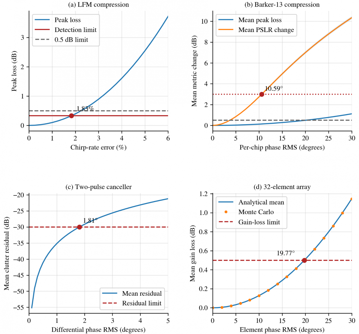
Interpolation of the LFM loss curve at that level gave a prescribed chirp-rate-error boundary of 1.83% and a half-power width increase of 0.98%. A standalone 0.5 dB peak-loss limit gave 2.25% and a 1.81% width increase as shown in Figure 2(a). The detection condition therefore reduced the chirp-rate boundary by approximately 18.6% in this model. These are deterministic mismatch boundaries; they are not Gaussian error standard deviations.
3.2 Barker-13 compression
For Barker-13, the mean peak loss reached 0.5 dB at σb = 20.14°, whereas the mean PSLR degradation reached 3 dB at σb= 10.59°. The sidelobe metric therefore governed this case. At the bracketing levels of 10° and 11°, the standard errors of mean PSLR degradation were 0.0351 and 0.0388 dB. The corresponding pointwise approximate 95% interval half-widths were 0.0689 and 0.0761 dB. The peak-loss standard errors at 20° and 21° were 0.00572 and 0.00631 dB as shown in Figure 2(b). These results support a mean-response boundary, not a bound satisfied by every realization. No confidence interval for the interpolated phase boundary itself was estimated.
To map σb to hardware sources, let chip j have phase error θj = ∑r hᵣurj, where hᵣ converts source error urj into radians. Then σb2 = hΣu hᵀ for each chip. The illustrative equal allocation assumes hᵣ = 1, four equal source variances, and independence both between sources and between chips. A phase term common to all chips rotates the compressed response but does not create the simulated sidelobe degradation. Consequently, the per-source value cannot be assigned to an oscillator without establishing its chip-to-chip covariance and transfer coefficients.
3.3 Moving-target-indication and active-array limits
The mean residual-power limit of 10⁻³ in Eq. (4) gave σΔφ = √[−2 ln(1 − 10⁻³/2)] = 0.0316267 rad = 1.81° as shown in Figure 2(c). If consecutive pulse errors are independent with equal variance, the corresponding per-pulse RMS phase error is 1.28°. For correlated pulses, the relation in Section 2.3 must be used instead. The limit refers to the aggregate phase difference at the canceller input, not directly to an oscillator phase-noise specification.
For the array, solving Eq. (5) with g = 10⁻⁰·⁰⁵ gave an element RMS phase error σa = 19.77° as shown in Figure 2(d). Monte Carlo interpolation gave 19.79°, and the maximum analytical-to-simulation difference over the sweep was below 0.003 dB. These results concern mean coherent power gain only. Their numerical comparison with the MTI boundary does not imply interchangeable phase specifications: the MTI variable is a temporal phase difference, whereas the array variable is an independent element phase error. No beam-pointing or sidelobe criterion was tested.
3.4 Illustrative allocation in normalized error coordinates
For an additive zero-mean error coordinate e = u₁ + u₂ + u₃ + u₄, the illustrative sensitivity row is h = [1, 1, 1, 1]. Independent equal sources have covariance Σu= (E²/4)I₄, where E denotes the aggregate RMS allowance, and I₄ is the identity matrix. Thus Var(e) = hΣu hᵀ = E², and each source has standard deviation E/2. Table 2 applies this arithmetic to the three phase-error coordinates. It gives 5.30° per source per chip for Barker-13, 0.91° per source for the MTI phase difference, and 9.89° per source per element for the array. Each value inherits the distribution and independence assumptions of its aggregate model.
Table 2. Aggregate boundaries and illustrative four-source shares
|
Error Coordinate |
Aggregate Boundary |
Illustrative Source Share |
|
Linear-frequency-modulated (LFM) chirp rate |
1.83% prescribed mismatch |
0.92% formal root-sum-square (RSS) only; ≤0.4575% worst-case bias |
|
Barker-13 chip phase |
10.59° root-mean-square (RMS) |
5.30° RMS per chip |
|
Moving-target indication (MTI) phase difference |
1.81° RMS |
0.91° RMS differential phase |
|
Array element phase |
19.77° RMS |
9.89° RMS per element |
The LFM row requires a different interpretation. Its 1.83% limit is a prescribed deterministic mismatch, so 0.92% is only a formal RSS share in a hypothetical random-error model. It does not ensure the stated packet detection probability. For four equal deterministic contributions with adverse signs, a sufficient worst-case allocation based on the reported 1.83% boundary is at most 1.83%/4 = 0.4575% per source. A random chirp-rate allocation would need its own distribution-aware detection calculation.
For a separate correlation illustration, suppose only sources 1 and 2 correlate 0.30, while all four source variances remain E²/4. The covariance is Σu= (E²/4)C, where the rows of C are [1, 0.30, 0, 0], [0.30, 1, 0, 0], [0, 0, 1, 0], and [0, 0, 0, 1]. This matrix is positive definite, with eigenvalues 1.30, 0.70, 1, and 1. The aggregate variance is hΣu hᵀ = (E²/4)(4 + 2 × 0.30) = 1.15E². The RMS factor is √1.15 = 1.0724. Scaling all source standard deviations by 1/√1.15 = 0.9325 restores E. For the three stochastic phase cases, the illustrative shares become 4.94°, 0.85°, and 9.22°. The factor 1.15 follows only from this covariance and sensitivity row; it is not a general correction for correlated hardware.
3.5 Applicability and limitations
The numerical cases establish which of the imposed metrics becomes active in each normalized model. The packet detection condition restricted LFM chirp-rate mismatch more than the 0.5 dB peak-loss rule. Mean PSLR degradation restricted Barker-13 chip phase error more than mean peak loss. MTI depended on differential temporal phase, while the array calculation concerned mean gain under independent element errors. The equal-share and correlation examples establish the associated covariance arithmetic, not a measured system-level allocation.
Other waveforms can be investigated by defining their nominal signals, error coordinates, processing operators, and required metrics. Prior waveform and calibration studies [4-6, 11-12] provide possible contexts for such work. Their applicability would need to be checked for the chosen architecture. MIMO, frequency-diverse arrays, and integrated sensing and communication were not simulated here, so no compatibility or performance claim is made for those systems.
Practical use requires separate treatment of calibration bias, random phase error, temporal correlation, and spatial correlation. A mean-gain limit does not constrain pointing or sidelobes. A confidence interval for an estimated mean does not provide a realization-level guarantee. Those additional criteria must be specified and verified before the illustrative source shares can be used as component requirements.
The evaluation was limited to the specified normalized LFM and Barker-13 signals, a two-pulse canceller, and an ideal broadside array. Measured component sensitivities, correlated chip-phase processes, non-Gaussian phase slips, amplifier memory, amplitude-to-phase conversion, oscillator spurs, quantization, and temperature dependence were not evaluated. A production study must retain the actual pulse duration, pulse-repetition interval, detector, array taper, calibration state, and hardware transfer functions. If the loss response is strongly nonlinear or an exceedance probability is prescribed, nonlinear uncertainty propagation is required instead of first-order loss linearization.
A mathematical framework was formulated to connect radar performance limits with signal-error coordinates and, where a stochastic source model is specified, source covariance. Its normalized examples showed that the governing constraint depends on the protected processing function. Detection loss, Barker-13 sidelobe degradation, MTI differential phase, and mean array gain therefore require distinct error definitions.
The equal-share calculations illustrate variance allocation under explicit unit-sensitivity and independence assumptions. The specified correlated-source example demonstrates how off-diagonal terms alter those shares. These results do not validate a complete radar or provide universal oscillator, clock, or array-channel specifications. Practical allocation requires measured source sensitivities and covariance, followed by verification of all applicable mean and probabilistic constraints in the nonlinear processing chain.
|
a |
normalized compressed-peak amplitude, dimensionless |
|
B |
waveform bandwidth, Hz |
|
C |
prescribed four-source correlation matrix, dimensionless |
|
Cj |
j-th radar-level characteristic |
|
E |
aggregate RMS allowance in an error coordinate |
|
Fj |
performance-to-metric mapping |
|
G |
hardware-error-to-metric mapping |
|
g |
normalized mean coherent array gain, dimensionless |
|
h |
source-to-error sensitivity row |
|
H(p) |
3-out-of-4 probability mapping, dimensionless |
|
I₄ |
four-dimensional identity matrix |
|
K |
chirp rate, Hz s⁻¹ |
|
k |
required number of detections |
|
m |
number of pulse decisions |
|
M |
nominal mainlobe interval |
|
N |
number of array elements |
|
Ns |
number of complex waveform samples |
|
pD, pF |
single-pulse detection and false-alarm probabilities |
|
PD, PF |
packet detection and false-alarm probabilities |
|
q |
vector of observable signal metrics |
|
R |
number of hardware-error sources |
|
rMTI |
normalized residual clutter power, dimensionless |
|
sd |
sample standard deviation of a simulated metric |
|
Sir |
sensitivity of metric i to source r |
|
Sφ(f) |
one-sided phase PSD, rad² Hz⁻¹ |
|
s₀, s |
nominal and perturbed complex waveforms |
|
T |
pulse duration, s |
|
Tr |
pulse-repetition interval, s |
|
t₀.₉₇₅,₁₁₉₉ |
Student t quantile for a pointwise 95% interval |
|
urj |
error from source r on chip j |
|
x |
vector of hardware errors |
|
zi |
i-th selected signal metric |
|
βir |
fraction of allowable metric variance assigned to source r |
|
δ |
normalized peak sidelobe ratio, dimensionless |
|
ΔCj |
admissible deterioration of Cj |
|
Δτ |
relative half-power width increase, dimensionless |
|
Δφₙ |
φₙ − φₙ₋₁, rad |
|
εK |
relative chirp-rate error, dimensionless |
|
η |
normalized square-law threshold, dimensionless |
|
θj |
phase error of chip j, rad |
|
ν |
signal-to-noise ratio, dimensionless |
|
ρ₁ |
lag-one phase correlation, dimensionless |
|
σa |
RMS element phase error, rad |
|
σb |
RMS per-chip phase error, rad |
|
σp |
RMS phase error of an individual pulse, rad |
|
Σu |
covariance of the illustrative source errors |
|
Σx |
hardware-error covariance matrix |
|
σΔφ |
RMS differential inter-pulse phase error, rad |
|
τ |
delay, s |
|
φₙ |
residual phase of pulse n, rad |
|
φℓ |
phase error of element ℓ, rad |
|
Abbreviations |
|
|
FMCW |
frequency-modulated continuous wave |
|
LFM |
linear frequency modulation |
|
MIMO |
multiple-input multiple-output |
|
MTI |
moving-target indication |
|
PCG64 |
permutedcongruentialgeneratorwith64-bitoutput |
|
PSLR |
peak sidelobe ratio |
|
PSD |
power spectral density |
|
RMS |
root-mean-square |
|
RSS |
root-sum-square |
|
SNR |
signal-to-noise ratio |
A. Numerical implementation
Calculations and figure generation used Python with NumPy 2.3.5, SciPy 1.17.0, and Matplotlib 3.10.8. Analytical responses and Monte Carlo simulations were evaluated for the normalized signal models.
Independent PCG64 generators, each initialized with seed 2026, were used for Barker-13 and the array. Each generator produced one complete standard-normal matrix, reused at all error levels. The array results therefore did not depend on the Barker draw count. Linear full-length convolution was used without circular wrapping.
The decibel conventions were as follows: compressed-peak loss is −20 log₁₀ of normalized amplitude; array loss is −10 log₁₀ of the mean normalized power; and MTI residual is 10 log₁₀ of mean normalized residual power. Barker PSLR degradation is calculated in decibels for each realization before averaging. Positive compression and array losses indicate deterioration in Figure 2.
Numerical verification checked packet-probability roots, nominal Barker PSLR, the analytical MTI and array boundaries, and agreement between Monte Carlo and analytical array means. These checks concern the normalized models within the scope defined in Section 3.5.
[1] Marcum, J.I. (1960). A statistical theory of target detection by pulsed radar. IRE Transactions on Information Theory, 6(2): 59-267. https://doi.org/10.1109/TIT.1960.1057560
[2] Siddiq, K., Hobden, M.K., Pennock, S.R., Watson, R.J. (2019). Phase noise in FMCW radar systems. IEEE Transactions on Aerospace and Electronic Systems, 55(1): 70-81. https://doi.org/10.1109/TAES.2018.2847999
[3] Tschapek, P., Körner, G., Carlowitz, C., Vossiek, M. (2022). Detailed analysis and modeling of phase noise and systematic phase distortions in FMCW radar systems. IEEE Journal of Microwaves, 2(4): 648-659. https://doi.org/10.1109/JMW.2022.3195574
[4] Bharadwaj, N., Chandrasekar, V. (2012). Wideband waveform design principles for solid-state weather radars. Journal of Atmospheric and Oceanic Technology, 29(1): 14-31. https://doi.org/10.1175/JTECH-D-11-00030.1
[5] Torres, S.M., Curtis, C.D., Schvartzman, D. (2017). Requirement-driven design of pulse compression waveforms for weather radars. Journal of Atmospheric and Oceanic Technology, 34(6): 1351-1369. https://doi.org/10.1175/JTECH-D-16-0231.1
[6] Azouz, A., Abosekeen, A., Nassar, S., Hanafy, M. (2021). Design and implementation of an enhanced matched filter for sidelobe reduction of pulsed linear frequency modulation radar. Sensors, 21(11): 3835. https://doi.org/10.3390/s21113835
[7] Thurn, K., Ebelt, R., Vossiek, M. (2013). Noise in homodyne FMCW radar systems and its effects on ranging precision. In 2013 IEEE MTT-S International Microwave Symposium Digest (MTT), Seattle, WA, USA, pp. 1-3. https://doi.org/10.1109/MWSYM.2013.6697654
[8] Siddiq, K., Watson, R.J., Pennock, S.R., Avery, P., Poulton, R., Martins, S. (2016). Analysis of sampling clock phase noise in homodyne FMCW radar systems. In 2016 IEEE Radar Conference (RadarConf), Philadelphia, PA, USA, pp. 1-4. https://doi.org/10.1109/RADAR.2016.7485302
[9] Levy, C., Pinchas, M., Pinhasi, Y. (2021). Coherent integration loss due to nonstationary phase noise in high-resolution millimeter-wave radars. Remote Sensing, 13(9): 1755. https://doi.org/10.3390/rs13091755
[10] Birkenhauer, C., Tschapek, P., Vossiek, M. (2024). Over-the-air phase noise spectral density measurement for FMCW radar sensors. IEEE Journal of Microwaves, 4(4): 733-741. https://doi.org/10.1109/JMW.2024.3471803
[11] Geiß, J., Sippel, E., Braunwarth, M., Vossiek, M. (2023). The impact of antenna array calibration errors on MIMO and multi-channel synthetic aperture radar imaging. IEEE Journal of Microwaves, 3(2): 635-654. https://doi.org/10.1109/JMW.2023.3254135
[12] González-Coma, J.P., Nocelo López, R., Núñez-Ortuño, J.M., Troncoso-Pastoriza, F. (2025). Beacon-based phased array antenna calibration for passive radar. Remote Sensing, 17(3): 490. https://doi.org/10.3390/rs17030490
[13] Mohammed, J.R. (2022). Elements selection for auxiliary array in the adaptive sidelobe canceller radar system. Periodica Polytechnica Electrical Engineering and Computer Science, 66(4): 406-414. https://doi.org/10.3311/PPee.20452
[14] Schmid, C.M., Schuster, S.S., Feger, R., Stelzer, A. (2013). On the effects of calibration errors and mutual coupling on the beam pattern of an antenna array. IEEE Transactions on Antennas and Propagation, 61(8): 4063-4072. https://doi.org/10.1109/TAP.2013.2259455