
Mohaimen M. Khudhur* | Sarmad A. Abbas | Ammar Dakhil
© 2026 The authors. This article is published by IIETA and is licensed under the CC BY 4.0 license (http://creativecommons.org/licenses/by/4.0/).
OPEN ACCESS
The Al-Gharraf River, traversing Wasit and Dhi Qar provinces in Iraq, is a major distributary of the Tigris River and an essential water resource for Wasit, Dhi Qar, and Basrah provinces. This study develops a two-dimensional depth-averaged hydrodynamic model of the Al-Gharraf River using the Saint-Venant equations integrated within the Hydrologic Engineering Center’s River Analysis System (HEC-RAS) framework. The model incorporates six major regulators and several distributary branches to simulate both longitudinal and transverse flow dynamics. Digital elevation models (DEMs) processed using Geographic Information Systems (GIS), together with field measurements collected during 2025, were employed to construct the model geometry and define boundary conditions. Calibration and verification were conducted using observed discharge and water level data collected at selected regulator stations along the river. Data from Regulator No. 1 were applied for model calibration, while verification was performed using an independent observation station located 17 km downstream from the upstream boundary. Model performance was evaluated using statistical indicators including Root Mean Square Error (RMSE), Mean Absolute Error (MAE), Nash-Sutcliffe Efficiency (NSE), and coefficient of determination (R²) The results demonstrated acceptable agreement between simulated and observed data, with NSE = 0.589, RMSE = 15.67 m³/s, MAE = 10.52 m³/s, and R² = 0.884. The simulation results indicate a relatively stable hydraulic system despite temporal variations in discharge caused by seasonal flow changes and regulator operations. The developed model provides a practical basis for future sediment transport and water quality studies and can support water resources management (WRM) and regulator operation optimization within the Al-Gharraf River system. However, model limitations related to DEM uncertainty, field data coverage, and assumptions associated with regulator operations should be considered in future applications.
Al-Gharraf River, two-dimensional hydrodynamic model, Saint-Venant equations, Hydrologic Engineering Center’s River Analysis System, hydraulic regulators, water surface elevation, manning’s roughness coefficient, Geographic Information Systems
Surface water denotes water bodies that accumulate on the Earth’s surface and are directly exposed to the atmosphere, including rivers, lakes, reservoirs, and estuaries. It represents a vital water resource, accounting for a significant proportion of global water use and serving as a primary source for drinking water, agriculture, industry, and ecological sustainability [1, 2].
River systems are intrinsically dynamic and influenced by both natural processes and human interventions. Modeling river hydraulics is particularly complex due to temporal and spatial variations in flow characteristics, as well as continuous changes in channel geometry [3]. Numerous studies in Iraq have utilized one-dimensional (1D) models to simulate the Al-Gharraf River, frequently overlooking the hydraulic influences of regulators and distributary branches, which are essential in regulating flow dynamics [3-5].
Previous research has demonstrated the advantages of two-dimensional (2D) modeling over simplified methodologies. Abed et al. [6] demonstrated that 2D simulations using the Hydrologic Engineering Center’s River Analysis System (HEC-RAS) provide more accurate predictions of flow velocity and Water surface elevation (WSE). Similarly, Al Jawei et al. [7] underscored the impact of upstream regulation on river discharge, whereas Kazem et al. [8] emphasized inefficiencies in water distribution along irrigation offtakes. Additional research has investigated water quality modeling and the comparison between 1D and 2D approaches, confirming the importance of advanced hydrodynamic representation.
This study aims to develop a comprehensive 2D hydrodynamic model of the Al-Gharraf River utilizing HEC-RAS, incorporating six regulators and major distributary branches along the river. The model integrates high-resolution topographic data obtained from SRTM and processed using Geographic Information Systems (GIS), along with field measurements collected in 2025. The study area extends from Sadr Al-Gharraf Regulator in Kut to Al-Bada’a Regulator in Dhi Qar [9-11].
The river flow is considered unsteady due to temporal variations in discharge caused by regulator operations and upstream releases. This research, in contrast to prior studies, encompasses the entire river reach, incorporating hydraulic structures and tributaries, thereby yielding a more accurate depiction of flow dynamics. The established model offers a robust basis for subsequent research on sediment transport and water quality in the Al-Gharraf River [12-14].
This study addresses an important research gap in hydraulic modeling of Iraqi rivers by developing a comprehensive two-dimensional hydrodynamic model for the entire Al-Gharraf River system. Unlike previous studies that focused on limited reaches or simplified one-dimensional approaches, the present model incorporates six major regulators, distributary branches, and recent field measurements within an integrated HEC-RAS framework. The integration of GIS-processed digital elevation model (DEM) data with detailed cross-sectional surveys collected during 2025 provides improved hydraulic representation and enhances the reliability of flow simulations along the river system.
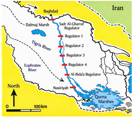
The Al-Gharraf River emanates from the Tigris River at the Kut Barrage, specifically at the Sadr Al-Gharraf Regulator, and flows southward between the Tigris and Euphrates Rivers until it reaches its terminal point at Al-Shatrah District in Dhi Qar Governorate [6, 8]. The river spans approximately 230 km and represents a major watercourse supplying irrigation demands across Wasit and Dhi Qar provinces. Along its course, the river passes through several key urban and agricultural regions, including Al-Mufaqiyah, Al-Hayy, Qalat Sukkar, and Al-Rifa’i, before reaching Al-Shatrah [8]. The WSE declines from approximately 17 m at the river’s origin to about 10 m at its downstream end, resulting in a mild longitudinal bed slope of approximately 0.0000475 [7, 15]. A system of control regulators has been established along the river to manage water levels and facilitate efficient irrigation distribution, comprising four primary regulators alongside the Sadr Al-Gharraf and Al-Bada’a regulators.
Figure 1. The Al-Gharraf River and the locations of the regulators
The initial regulator is positioned south of the Sadr Al-Gharraf Regulator and upstream of Al-Hayy District; the second is situated between Al-Hayy and Qalat Sukkar; the third is located north of Qalat Sukkar; and the fourth is found south of Al-Rifa’i City. These hydraulic structures were engineered to facilitate the expansion of irrigated agriculture and to regulate flow conditions, with design discharges of approximately 450, 350, 300, and 250 m³/s, respectively. Figure 1 illustrates the longitudinal distribution of the six major regulators along the Al-Gharraf River, including Sadr Al-Gharraf Regulator, Regulators No. 1-4, and Al-Bada’a Regulator. The coordinates and hydraulic characteristics of each regulator were verified and consistently presented throughout the manuscript to improve clarity and reproducibility [8, 16].
The Al-Gharraf River is categorized as a shallow water system due to its width-to-depth ratio surpassing 10. A depth-averaged 2D hydrodynamic model was utilized to simulate changes in hydraulic properties across the horizontal plane (longitudinal and transverse directions), employing HEC-RAS [4, 17, 18].
The term “2D depth-averaged” refers to a hydraulic modeling approach in which the flow variables are averaged over the water depth, allowing simulation of horizontal flow behavior while reducing computational complexity. The Diffusion Wave solver in HEC-RAS is a simplified hydrodynamic solution approach that improves computational efficiency under gradually varied flow (GVF) conditions.
While the two-dimensional Diffusion Wave approach is the default solver in HEC-RAS and offers computational efficiency and improved numerical stability, the full two-dimensional momentum equations (2D Saint-Venant equations) were employed in this study due to their capability to represent a wider range of hydraulic conditions with higher accuracy. Both methodologies are based on an implicit finite volume solution scheme [2, 11, 13, 14]. Moreover, the variable time-step option in HEC-RAS enables automatic adjustment of the computational time step according to the selected Courant number, thereby ensuring numerical stability and accuracy [14, 18].
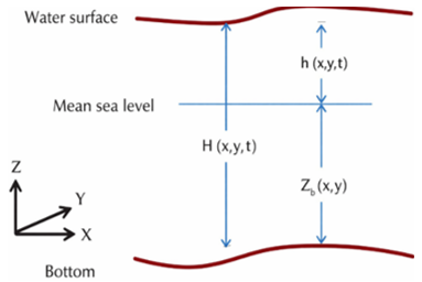
The schematic representation of the water surface elevation, bed elevation, and total water depth is illustrated in Figure 2.
Figure 2. Schematic geometry of water and bed elevation
The governing two-dimensional Saint-Venant equations used in this study are expressed as follows [11, 17, 18]:
$\frac{\partial H}{\partial t}+\frac{\partial(H u)}{\partial x}+\frac{\partial(H v)}{\partial y}=q$ (1)
$\begin{gathered}\frac{\partial u}{\partial t}+u \frac{\partial u}{\partial x}+v \frac{\partial u}{\partial y}-f_c v=-g \frac{\partial h}{\partial x}+\frac{1}{H} \frac{\partial}{\partial x}\left(v_{t, x x} H \frac{\partial u}{\partial x}\right)+\frac{1}{H} \frac{\partial}{\partial y}\left(v_{t, y y} H \frac{\partial u}{\partial y}\right)-\frac{\tau_{b, x}}{\rho R}-\frac{\tau_{s, x}}{\rho H}\end{gathered}$ (2)
$\begin{gathered}\frac{\partial v}{\partial t}+u \frac{\partial v}{\partial x}+v \frac{\partial v}{\partial y}+f_c u=-g \frac{\partial h}{\partial y}+\frac{1}{H} \frac{\partial}{\partial y}\left(v_{t, x x} H \frac{\partial v}{\partial x}\right)+\frac{1}{H} \frac{\partial}{\partial y}\left(v_{t, y y} H \frac{\partial v}{\partial y}\right)-\frac{\tau_{b, y}}{\rho R}-\frac{\tau_{s, y}}{\rho H}\end{gathered}$ (3)
where, $t$ is time. $H=h+z_b$ is the total water depth, where $h$ is the WSE and $z_b$ is the bed elevation. $u$ and $v$ are the velocity components in the x- and $y$-directions, respectively. $q$ is the source/sink flux, $g$ is the gravitational acceleration, $v_{t, x x}$ and $v_{t, y y}$ are the horizontal eddy viscosity coefficients, $\tau_{b, x}$ and $\tau_{b, y}$ are the bed shear stresses, $\tau_{s, x}$ and $\tau_{s, y}$ are the surface wind stresses, $R$ is the hydraulic radius, and $f_c$ is the Coriolis parameter.
4.1 Digital elevation model
DEMs are essential topographic datasets widely used in hydrodynamic modeling and flood inundation analysis. They represent the Earth’s surface as a raster grid, where each cell contains an elevation value corresponding to ground level, excluding vegetation and man-made structures [9, 19].
DEMs play a critical role in engineering and environmental applications, particularly in water resources management (WRM), where accurate elevation data are required and typically integrated within GIS [9, 10].
In this study, topographic data were obtained from the freely available Earth Explorer platform. The datasets were processed in raster format using the Space Shuttle Radar Topography Mission (SRTM Arc-Second Global), which is considered one of the most reliable global DEM sources [15, 20]. Although the integration of surveyed cross-sections improved river channel representation, uncertainties associated with the vertical accuracy of SRTM DEM data may still affect floodplain representation and local hydraulic simulation results, particularly in low-gradient river systems such as the Al-Gharraf River.
4.1.1 Digital elevation model modification
To ensure accurate flow direction extraction, the DEM must be free of depressions, as these can introduce significant errors in the derived drainage network. Therefore, the Hydrology tools within the Spatial Analyst extension in ArcGIS were applied to fill surface depressions and generate a hydrologically corrected DEM suitable for further analysis [10, 20].
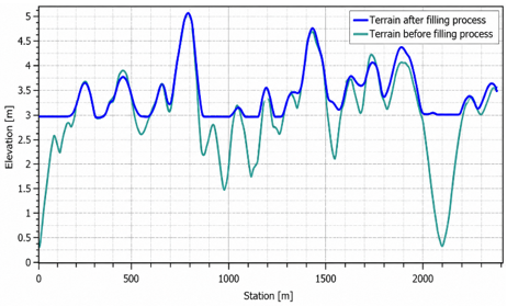
Previous studies indicate that approximately 0.9% to 4.7% of DEM cells may be classified as depressions requiring correction to enhance the reliability of hydrological modeling. Figure 3 illustrates examples of depressions that were identified and filled during the preprocessing stage [20, 21].
Figure 3. Terrain profile before and after filling process
4.1.2 Including channel bathymetry into terrain
An accurate representation of terrain is fundamental for developing a reliable hydraulic model. However, DEMs typically lack riverbed elevation data, as most remote sensing techniques are unable to penetrate the water surface [9, 21].
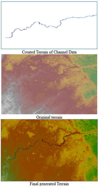
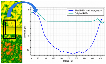
To address this limitation, river cross-section data were incorporated to reconstruct the riverbed topography using HEC-RAS 6.1. A GeoTIFF terrain file was generated from the cross-sectional data and subsequently integrated with the original DEM within RAS Mapper, resulting in a refined and comprehensive terrain model of the study area [10, 11].
The SRTM DEM used in this study has a spatial resolution of 30 m. To improve terrain representation within the river channel, the surveyed cross-sectional bathymetry data were interpolated and converted into a GeoTIFF terrain layer using HEC-RAS and RAS Mapper tools. The generated bathymetric terrain was subsequently merged with the original DEM to produce a hydraulically corrected terrain model suitable for two-dimensional flow simulation.
This approach enabled a more accurate definition of the geometric characteristics of the Al-Gharraf River, as illustrated in Figures 4 and 5 [9, 18].
Figure 4. Digital elevation model (DEM) developed stages
Figure 5. Properties of the final generated digital elevation model (DEM)
4.2 Cross sections
River cross-sections constitute a fundamental input for hydraulic model development. Due to the absence of such data for the Al-Gharraf River in the official databases of Wasit and Dhi Qar governorates, detailed field surveys were conducted and the collected data were integrated into the DEM [9, 21].
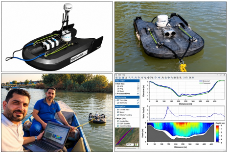
In this study, cross-sectional measurements were obtained using the Son Tek River Surveyor Live (Version 4.1), which provides high-resolution and accurate estimates of river depth and channel width. A survey boat was employed to access multiple measurement locations across the river, enabling efficient and safe data acquisition along both banks and the main channel, as illustrated in Figure 6.
The spacing of the surveyed cross-sections was not completely uniform along the river reach. Higher cross-section density was applied near regulators, distributary branches, and hydraulically sensitive locations to improve geometric and hydraulic representation. The cross-sections were surveyed approximately perpendicular to the flow direction, and the SonTek River Surveyor system provided high-resolution bathymetric measurements suitable for two-dimensional hydraulic modeling.
Figure 6. Site measuring instruments
A total of 170 cross-sections were incorporated into the model, significantly enhancing the representation of channel geometry and improving the accuracy of the simulated topographic variations along the river reach.
4.3 Generation of land-cover data from satellite images
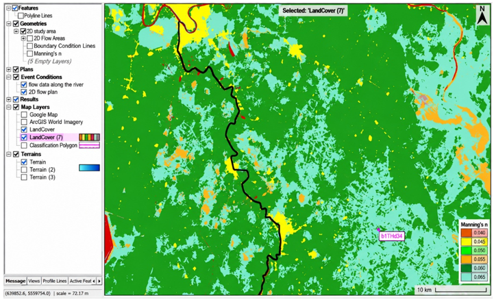
In 2D hydrodynamic modeling, Manning’s roughness coefficient (n) is commonly linked to land cover classifications in HEC-RAS. Its values are influenced by surface characteristics, permeability, flow depth, and channel geometry [11, 18].
While extensive research has focused on Manning’s n in 1D channels, studies addressing its estimation in 2D modeling domains remain relatively limited [2, 17].
The RAS Mapper tool allows the integration of land cover data with topographic information, enabling the assignment of spatially distributed Manning’s n values based on land use categories (Figure 7) [10, 11]. The adopted roughness ranges for each class were defined according to the National Land Cover Database (NLCD), as summarized in Table 1 [22].
Figure 7. Region classification of land cover layer
Table 1. Roughness coefficient for land cover classification of National Land Cover Database (NLCD)
|
NLCD Code |
Land Cover Definition |
Range of Manning's n Value |
|
11 |
Open Water |
0.025–0.05 |
|
21 |
Developed, Open Space |
0.03–0.05 |
|
22 |
Developed, Low Intensity |
0.08–0.12 |
|
23 |
Developed, Medium Intensity |
0.06–0.14 |
|
24 |
Developed, High Intensity |
0.12–0.2 |
|
31 |
Barren Land (Rock/Sand/Clay) |
0.023–0.03 |
|
41 |
Deciduous Forest |
0.1–0.16 |
|
42 |
Evergreen Forest |
0.1–0.16 |
|
43 |
Mixed Forest |
0.1–0.16 |
|
52 |
Shrub/Scrub |
0.07–0.16 |
|
71 |
Grassland/Herbaceous |
0.07–0.16 |
|
81 |
Pasture/Hay |
0.025–0.05 |
|
82 |
Cultivated Crops |
0.025–0.05 |
|
90 |
Woody Wetlands |
0.045–0.15 |
|
95 |
Emergent Herbaceous Wetlands |
0.05–0.085 |
4.4 Two-dimensional flow area and meshing
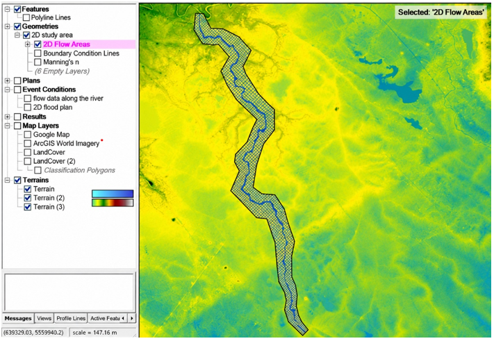
The 2D flow area was delineated within the HEC-RAS environment to include the river channel and adjacent floodplain extending from Kut to Al-Shatrah, as illustrated in Figure 8.
Figure 8. Two-dimensional (2D) flow area perimeter and mesh details in different regions
An initial computational mesh with a uniform cell size was generated to cover the entire study domain. To improve the representation of flow characteristics, the mesh was refined along the main river course using break lines.
Additional refinement was applied to narrow branches along the riverbanks using refinement polygons, ensuring higher numerical accuracy in these critical areas. As a result, the final mesh consisted of 52,944 computational cells.
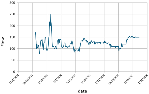
Boundary conditions were defined to represent the hydrological inputs and outputs of the two-dimensional HEC-RAS model for the Al-Gharraf River. The discharge hydrograph recorded at the Sadr Al-Gharraf Regulator (Kut City) was applied as the upstream boundary condition, representing river inflow (Figure 9).
Figure 9. Observed flow for upstream boundary conditions at the Sadr Al-Gharraf Regulator
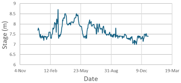
At the downstream boundary, the stage hydrograph recorded at Al-Bada’a Regulator in Dhi Qar Governorate was used to represent outflow conditions.
A daily time series covering one hydrological year (December 2024 to November 2025) was employed for both discharge and water level data to capture temporal flow variability and enhance model reliability. The dataset is summarized in Table 2 and illustrated in Figure 10.
Table 2. Station location of data collected during simulation time
|
Station |
Location Coordinate |
Data Type |
Purpose |
|
|
N |
E |
|||
|
Regulator Sadr Al-Gharraf |
32° 30΄08 ̎ |
45° 48΄28 ̎ |
Flow hydrograph |
Upstream BC |
|
17 km from upstream end |
32° 23΄12 ̎ |
45° 33΄17 ̎ |
Velocity hydrograph |
verification |
|
Regulator No. (1) |
32° 10΄49 ̎ |
46° 01΄23 ̎ |
Stage hydrograph |
Calibration |
|
Regulator No. (2) |
31° 59΄43 ̎ |
45° 58΄45 ̎ |
Stage hydrograph |
Hydraulic monitoring station |
|
Regulator No. (3) |
31° 53΄00 ̎ |
46° 03΄26 ̎ |
Stage hydrograph |
Hydraulic monitoring station |
|
Regulator No. (4) |
31° 39΄30 ̎ |
46° 06΄14 ̎ |
Stage hydrograph |
Hydraulic monitoring station |
|
Al-Bada’a Regulator |
31° 26΄45 ̎ |
46° 10΄33 ̎ |
Stage hydrograph |
Downstream BC |
Figure 10. Observed water stages for downstream boundary conditions at Al-Bada’a Regulator
The major distributary branches, hydraulic regulators, and irrigation withdrawal points were explicitly incorporated into the HEC-RAS model based on their actual locations and hydraulic characteristics along the Al-Gharraf River.
Model calibration involves adjusting model parameters to minimize discrepancies between simulated and observed data, while validation assesses model performance using independent datasets [12].
Model performance was evaluated using standard statistical indicators, including Mean Absolute Error (MAE), Root Mean Square Error (RMSE), and Nash-Sutcliffe Efficiency (NSE) [13].
$M A E=\frac{1}{N} \sum_{i=1}^N\left|S_i-O_i\right|$ (4)
$R M S E=\sqrt{\frac{\sum_i^N\left(S_i-O_i\right)^2}{N}}$ (5)
$N S E=1-\frac{\sum_i^N\left(S_i-O_i\right)^2}{\sum_i^N\left(S_i-O_o\right)^2}$ (6)
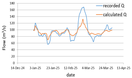
where, N = number of observed and simulated pairs, Oi = observed data, Si = simulated data, and Oo = mean of the observed data. To verify model reliability, simulated discharge values were compared with observed data along the Al-Gharraf River during the period from late December 2024 to early April 2025. The results showed good agreement, with the simulated data capturing the overall temporal trends of the observed discharge. Minor deviations in peak and low values were observed, which are typical in hydraulic modeling due to numerical and boundary condition limitations.
Statistical indicators confirmed acceptable model performance, with a correlation coefficient (r) of 0.94 and a coefficient of determination (R²) of 0.884, indicating that approximately 88% of the observed variability was explained by the model. The NSE value was 0.589, with RMSE = 15.67 m³/s and MAE = 10.52 m³/s. Additionally, the PBIAS value of −1.47% indicates minimal systematic bias.
Overall, the model demonstrates satisfactory performance and provides a useful tool for hydraulic analysis and scenario evaluation [14].
6.1 Model calibration and verification using observed and simulated data
Several Manning’s roughness coefficients were tested, and n = 0.05 was selected because it provided the best agreement between simulated and observed discharge, based on RMSE, MAE, and NSE (Table 3 and Figure 11). The calibrated value (n = 0.05) represents the effective roughness coefficient of the main river channel used during the calibration process and should not be interpreted as a uniform roughness value for the entire computational domain.
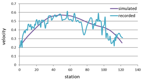
Model calibration was performed using discharge hydrograph data recorded at Regulator No. 1 for the period from 1 January to 1 June 2025. Model verification was conducted using observed velocity data collected at a monitoring station located 17 km downstream from the upstream boundary. The verification results are presented in Table 4 and Figure 12.
Table 3. Model performances statistic during calibration
|
n Value |
Statistical Analysis Method |
||
|
RMSE (m³/s) |
MAE (m³/s) |
NSE |
|
|
0.06 |
27.2 |
20 |
0.918 |
|
0.05 |
12.7 |
10 |
0.988 |
|
0.04 |
19.7 |
16 |
0.915 |
|
0.03 |
32.7 |
25 |
0.857 |
Table 4. Statistical performance indicators of the model during verification
|
Station |
Statistical Analysis Method |
||
|
RMSE (m/s) |
MAE (m/s) |
NSE |
|
|
17km from upstream end |
0.223 |
0.185 |
0.928 |
Figure 11. Graphical comparison between observed and simulated data at Regulator No. 1 station
Figure 12. Comparison of observed and simulated velocity at the station located 17 km downstream from the upstream boundary
Further verification was carried out by comparing simulated and observed discharge along the Al-Gharraf River for the period from late December 2024 to early April 2025. The comparison between observed and simulated discharge is presented in Figure 13, showing that the model successfully captures the overall temporal trends, despite minor deviations in peak and low values, which are commonly expected due to numerical diffusion and boundary condition simplifications.
Figure 13. The comparison between the recorded discharge (Observed Q) and the calculated discharge (Simulated Q)
The calibration and verification stations were selected to represent different hydraulic conditions along the Al-Gharraf River, including reaches influenced by hydraulic regulators and varying discharge conditions. Some discrepancies between observed and simulated results may be associated with numerical diffusion effects, uncertainties in boundary condition measurements, and lateral withdrawals occurring along the river system.
Statistical indicators confirmed satisfactory model performance, with a correlation coefficient (r = 0.94) and coefficient of determination (R² = 0.884), indicating that approximately 88% of the observed variability was explained by the model. The NSE value (0.589), along with RMSE (15.67 m³/s) and MAE (10.52 m³/s), further supports model reliability. The low PBIAS value (−1.47%) indicates minimal systematic bias, as summarized in Table 5.
Although the model demonstrated acceptable agreement with the observed data, some deviations were observed during peak discharge periods. These discrepancies may be attributed to uncertainties in boundary condition measurements, lateral withdrawals, DEM accuracy limitations, and numerical simplifications within the two-dimensional model. Therefore, the NSE value of 0.589 should be interpreted as acceptable model performance under the complex hydraulic conditions of the Al-Gharraf River system rather than excellent agreement
Overall, the model demonstrates acceptable accuracy and provides a useful tool for hydraulic analysis and scenario evaluation [23].
Table 5 summarizes the overall statistical performance of the model based on the comparison between observed and simulated discharge data during the period from late December 2024 to early November 2025.
Table 5. Statistical performance indicators
|
Indicator |
Value |
Interpretation |
|
Correlation coefficient (r) |
0.94 |
Very strong correlation |
|
Coefficient of determination (R²) |
0.884 |
88.4% of observed variance explained |
|
Nash–Sutcliffe Efficiency (NSE) |
0.589 |
Acceptable model performance |
|
Root Mean Square Error (RMSE) |
15.67 m³/s |
Moderate error relative to peak flows |
|
Mean Absolute Error (MAE) |
10.52 m³/s |
Average deviation between series |
|
Percent Bias (PBIAS) |
−1.47% |
Very small underestimation bias |
6.2 Water surface elevation and discharge results
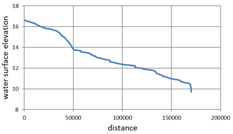
Figure 14 illustrates the longitudinal profile of WSE along the Al-Gharraf River on 10 February 2025. The horizontal axis represents the stationing distance along the river, while the vertical axis shows the WSE relative to a reference datum.
Figure 14. Water surface elevation (WSE) along the Al-Gharraf River on 10 Feb. 2025
At the upstream boundary, the WSE is approximately 16.6 m and gradually decreases to about 10.5 m over a distance of nearly 165 km downstream. This gradual decline reflects the longitudinal energy slope governed by gravity and flow resistance, with an overall monotonic trend indicating subcritical flow conditions typical of lowland rivers.
Localized variations in the slope are observed, particularly between 35–50 km and, to a lesser extent, between 110-130 km. These changes may be attributed to variations in channel geometry, bed slope, roughness, or the presence of hydraulic structures [24]. In contrast, the remaining reaches exhibit a smooth and gradual profile, indicating steady GVF [25]. These localized variations may also indicate zones of hydraulic control where minor changes in geometry or regulator operations influence the energy gradient, leading to temporary adjustments in flow conditions along the river reach [26].
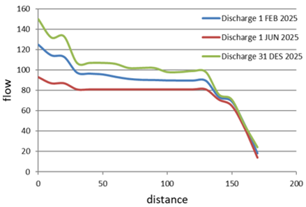
Figure 15. Longitudinal distribution of flow rate along the Al-Gharraf River on 1 Feb. 2025
Figure 15 presents the longitudinal variation of discharge along the river. The discharge starts at approximately 125 m³/s at the upstream boundary and decreases to about 95 m³/s within the first 40–50 km, likely due to lateral abstractions and irrigation withdrawals.
Between 50 km and 120 km, the discharge remains relatively stable, ranging between 88–92 m³/s, indicating a near-balanced hydraulic condition. Beyond 130 km, a significant drop occurs, with discharge decreasing to approximately 45 m³/s near the downstream end. This reduction suggests substantial water extraction, distributary branching, or operational control structures.
The decreasing discharge trend is consistent with variations in velocity and WSE, in accordance with the continuity equation (Q = A⋅V) [17]. Overall, the results indicate a non-conservative flow system influenced by lateral withdrawals and hydraulic controls, which govern the spatial variability of flow along the river.
This behavior highlights the significant impact of irrigation demands and branch diversions on the river system, indicating that water management practices play a key role in controlling downstream flow availability [27].
The observed variations in discharge and velocity along the river are strongly influenced by regulator operations and distributary branches. Hydraulic regulators contribute to stabilizing upstream water levels while simultaneously controlling downstream discharge and flow velocity distribution along different river reaches.
6.3 Velocity results
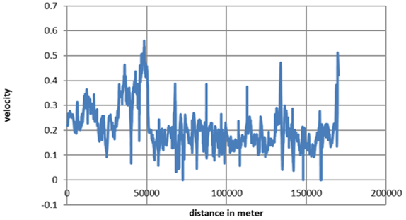
Figure 16 illustrates the longitudinal distribution of flow velocity along the centerline of the Al-Gharraf River at the simulation time “01FEB2025 00:00:00.” The velocity generally ranges between 0.15 and 0.35 m/s along most of the river reach, reflecting subcritical flow conditions typical of low-gradient alluvial channels.
Figure 16. Velocity distribution of the study area at different locations
A noticeable increase in velocity is observed between 30,000 m and 50,000 m, where values reach approximately 0.5–0.65 m/s. This increase corresponds to a steeper water surface gradient identified in the WSE profile and indicates localized changes in channel geometry, flow area, or hydraulic resistance. Overall, the spatial variability in velocity reflects non-uniform flow conditions influenced by hydraulic and geometric factors.
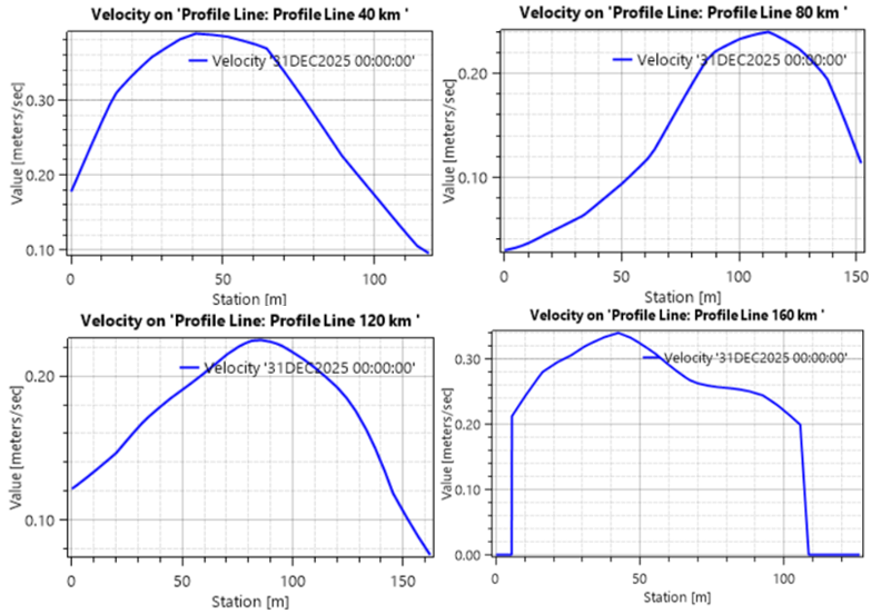
Figure 17 presents the transverse velocity distribution at selected locations along the river (e.g., 40, 80, 120, and 160 km). The profiles show that velocities are lowest near the channel boundaries due to frictional effects and reach maximum values within the main flow region.
Figure 17. The transverse velocity distribution across the channel at 4 different locations along the flow path: 40 km, 80 km, 120 km and 160 km
Variations in the shape of the velocity profiles along the river indicate changes in flow conditions and channel geometry. These variations play an important role in mixing processes and influence longitudinal dispersion characteristics [2].
6.4 Regulator results
The evaluation of regulator performance is essential for understanding the hydraulic behavior of the system, its operational efficiency, and its influence on flow stability. This assessment is based on the analysis of key hydraulic indicators derived from the numerical model results.
Regulator No. 1 was selected as a representative hydraulic structure for detailed analysis because of the availability of continuous operational observations. The remaining regulators demonstrated generally similar hydraulic behavior within the developed model, with variations mainly associated with local discharge conditions and operational control.
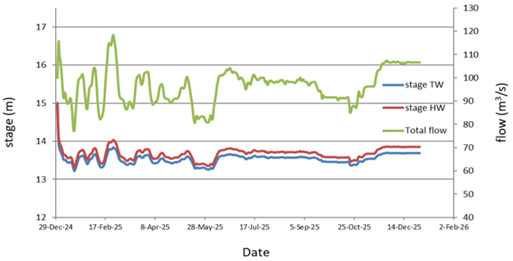
Figure 18 presents the temporal variation of hydraulic parameters over the year 2025. The left vertical axis represents water level (stage) in meters, while the right vertical axis corresponds to total discharge (m³/s), and the horizontal axis indicates the time progression.
The figure includes three main variables: headwater stage (HW), tailwater stage (TW), and total discharge. The HW and TW series exhibit closely aligned trends throughout the monitoring period, with a consistently small head difference ranging between approximately 0.2 and 0.5 m. This behavior indicates a low-head hydraulic system operating under well-controlled conditions [12].
Figure 18. A detailed hydraulic analysis of Regulator No. 1
Overall, the results indicate that the regulator shows stable operational behavior under the simulated conditions, maintaining stable water levels despite considerable variations in discharge. The small and consistent head difference further confirms stable and well-controlled operational conditions. This small head difference suggests that the regulator results in energy dissipation and maintains hydraulic equilibrium between upstream and downstream conditions.
An initial decline in water levels is observed, where the HW decreases from approximately 15 m to about 13.5 m. Subsequently, both HW and TW stabilize and fluctuate within a relatively narrow range for the remainder of the period, reflecting effective water level regulation.
In contrast, the discharge shows significant temporal variability, with higher and more fluctuating values during the winter and spring seasons, followed by a noticeable reduction in early summer. The flow then stabilizes before increasing again toward the end of the year. This pattern reflects seasonal hydrological variability driven by upstream inflows and climatic conditions.
These fluctuations indicate that the regulator operation adapts to varying inflow conditions, ensuring stable upstream water levels despite significant seasonal changes in discharge.
Based on the hydraulic analysis of the Al-Gharraf River using the two-dimensional HEC-RAS model, the following conclusions can be drawn:
1. The developed hydraulic model indicated acceptable agreement between simulated and observed data, confirming its ability to represent the hydraulic behavior of the river.
2. The optimal Manning’s roughness coefficient (n) was found to be 0.05, which provided the best fit according to the statistical performance indicators.
3. The longitudinal water surface profile demonstrated a gradual decline along the river reach under subcritical flow conditions, reflecting the natural hydraulic slope of the channel.
4. The findings indicated a progressive reduction in discharge along the river due to lateral withdrawals and irrigation demands, with relatively stable flow conditions in some reaches.
5. The analysis of regulators indicated that these structures effectively maintain upstream water levels and regulate downstream discharge, contributing to hydraulic stability along the Al-Gharraf River.
6. The developed model can serve as a useful tool for supporting WRM and optimizing regulator operation along the Al-Gharraf River.
7. The findings provide a practical basis for future studies related to sediment transport and water quality assessment under varying hydraulic conditions.
8. The developed model can also support operational decision-making related to regulator management and irrigation water distribution under different hydrological conditions, including high-flow and low-flow periods.
Although the developed model demonstrated acceptable performance in simulating the hydraulic behavior of the Al-Gharraf River, the results remain subject to uncertainties associated with DEM accuracy, bathymetric representation, lateral withdrawals, and seasonal irrigation variations. Therefore, the model should be considered a supportive hydraulic analysis tool within the limitations of the available field data and modeling assumptions adopted in this study.
[1] Behzadi, F., Wasti, A., Steissberg, T.E., Ray, P.A. (2022). Vulnerability assessment of drinking water supply under climate uncertainty using a river contamination risk (RANK) model. Environmental Modelling & Software, 150: 105294. https://doi.org/10.1016/j.envsoft.2021.105294
[2] Fan, C., Ko, C.H., Wang, W.S. (2009). An innovative modeling approach using Qual2K and HEC-RAS integration to assess the impact of tidal effect on river water quality simulation. Journal of Environmental Management, 90(5): 1824-1832. https://doi.org/10.1016/j.jenvman.2008.11.011
[3] Al-Mahmood, H.K., Al-Sayaab, H.A., Al-Miahi, D.S.B., M, A.B., Mutasher, W.R. (2011). One dimensional model to study hydrodynamics properties for north part of Shatt AL Arab River (South Iraq). Basrah Journal of Science, 28(1): 1-14. https://faculty.uobasrah.edu.iq/uploads/publications/1682580518.pdf.
[4] Najm, A.T. (2017). Applications of two-dimensional surface flow modelling for Shatt Al-Arab River in civil engineering / water resources. University of Basrah.
[5] Abbas, A.H.A.K. (2017). Application of a hydrodynamic HEC-RAS model for Shatt Al-Arab River. Muthanna Journal of Engineering and Technology, 2: 11-22. https://muthjet.mu.edu.iq/wp-content/uploads/2022/07/Application-of-a-Hydrodynamic-HEC-RAS-Model-For-Shatt-Al-Arab-River-1.pdf.
[6] Abed, B.Sh., Daham, M.H., Al-Thamiry, H.A. (2020). Assessment and modelling of water quality along Al-Gharraf River (Iraq). Journal of Green Engineering, 10(12): 13565-13579.
[7] Al Jawei, A.Y., Ghafouri, H.R., Abood, A.R. (2023). Hydrological impact of Ilisu Dam on Al-Gharraf River in southern of Iraq using MIKE11 hydrodynamic model. IOP Conference Series: Earth and Environmental Science, 1232(1): 12020. https://doi.org/10.1088/1755-1315/1232/1/012020
[8] Kazem, F.H., Maatoq, J.S., Wahad, M.S. (2024). Evaluation of hydraulic structures for agricultural discharge optimization. Civil Engineering Journal, 10(5): 1513-1523.
[9] Merwade, V., Cook, A., Coonrod, J. (2008). GIS techniques for creating river terrain models for hydrodynamic modeling and flood inundation mapping. Environmental Modelling & Software, 23(10-11): 1300-1311. https://doi.org/10.1016/j.envsoft.2008.03.005
[10] Pandya, K.H., Vadodaria, G.P., Prakash, I. (2018). Use of ArcGIS to extract River Geometry as an input to HEC-RAS for Flood Modelling. International Journal of Innovative Research in Technology, 4(12): 696-699. https://www.academia.edu/42141610/Use_of_ArcGIS_to_extract_river_geometry_as_an_input_to_HEC_RAS_for_Flood_Modelling.
[11] Brunner, G.W. (2010). HEC-RAS river analysis system: Hydraulic reference manual. US Army Corps of Engineers, Institute for Water Resources, Hydrologic Engineering Center.
[12] Abdullah, A.D. (2016). Modelling Approaches to Understand Salinity Variations in a Highly Dynamic Tidal River. London, CRC Press. https://doi.org/10.1201/9781315115948
[13] Krause, P., Boyle, D.P., Bäse, F. (2005). Comparison of different efficiency criteria for hydrological model assessment. Advances in Geosciences, 5: 89-97. https://doi.org/10.5194/adgeo-5-89-2005
[14] Vedmani, R.K.P., Pandey, V.K. (2020). Calibration and validation of HEC-RAS model for minor command in coastal region. International Journal of Current Microbiology and Applied Sciences, 9(2): 664-678. https://doi.org/10.20546/ijcmas.2020.902.082
[15] Kadhim, A.A. (2018). Measuring and modeling the effects of sea level rise on near-coastal riverine regions: A geospatial comparison of the Shatt Al-Arab River in southern Iraq with the Mississippi River Delta in southern Louisiana, USA. Michigan State University.
[16] Hamdan, A.N. (2016). Simulation of salinity intrusion from Arabian Gulf to Shatt Al-Arab River. Basrah Journal for Engineering Science, 16(1): 28-32. https://doi.org/10.33971/bjes.16.1.5
[17] Marvin, J., Wilson, A.T. (2016). One dimensional, two dimensional and three dimensional hydrodynamic modeling of a Dyked Coastal River in the bay of fundy. Journal of Water Management Modeling. https://doi.org/10.14796/JWMM.C404
[18] Alzahrani, A.S. (2017). Application of two-dimensional hydraulic modeling in riverine systems using HEC-RAS. University of Dayton. http://rave.ohiolink.edu/etdc/view?acc_num=dayton1493135117254329.
[19] Croneborg, L., Matera, M., McKeown, D., van Aardt, J. (2015). Digital elevation models. International Bank for Reconstruction and Development, pp. 1-89. https://www.gfdrr.org/sites/default/files/publication/Digital-Elevation-Models-10-23-15-web.pdf.
[20] Tarboton, D.G., Bras, R.L., Rodriguez-Iturbe, I. (1991). On the extraction of channel networks from digital elevation data. Hydrological Processes, 5(1): 81-100. https://doi.org/10.1002/hyp.3360050107
[21] Gichamo, T.Z., Popescu, I., Jonoski, A., Solomatine, D. (2012). River cross-section extraction from the ASTER global DEM for flood modeling. Environmental Modelling & Software, 31: 37-46. https://doi.org/10.1016/j.envsoft.2011.12.003
[22] Nyaupane, N., Bhandari, S., Rahaman, M.M., et al. (2018). Flood frequency analysis using generalized extreme value distribution and floodplain mapping for hurricane harvey in Buffalo Bayou. In World Environmental and Water Resources Congress 2018: Watershed Management, Irrigation and Drainage, and Water Resources Planning and Management, Reston, VA: American Society of Civil Engineers, pp. 364-375. https://doi.org/10.1061/9780784481400.034
[23] Al Murib, M. (2018). Hydrodynamic and water quality modeling of the Tigris River system in Iraq using CE-QUAL-W2. Doctoral Dissertation, Portland State University.
[24] Al-Asadi, S.A., Alhello, A.A., Ghalib, H.B., Muttashar, W.R., Al-Eydawi, H.T. (2022). Seawater intrusion into Shatt Al-Arab River, Northwest Arabian/Persian Gulf. Journal of Applied Water Engineering and Research, 11(2): 289-302. https://doi.org/10.1080/23249676.2022.2113460
[25] Al-Azzawi, S.N., Khudair, K.M. (2001). A finite element model to simulate the hydrodynamics of Shatt Al-Basrah Canal and Khour Al-Zubair Estuary. Journal of Engineering, 7(2): 283-308.
[26] Lafta, A.A. (2022). Investigation of tidal asymmetry in the Shatt Al-Arab River Estuary, Northwest of Arabian Gulf. Oceanologia, 64(2): 376-386. https://doi.org/10.1016/j.oceano.2022.01.005
[27] Hamdan, A., Dawood, A., Naeem, D. (2018). Assessment study of water quality index (WQI) for Shatt Al-Arab River and Its Branches, Iraq. In MATEC Web of Conferences, The 3rd International Conference on Buildings, Construction and Environmental Engineering, BCEE3-2017, Sharm el-Sheikh, Egypt, 162: 5005. https://doi.org/10.1051/matecconf/201816205005