
Sugacini Mohankumar* | Ananda Babu Sairam | Ranjith Venugopal
© 2026 The authors. This article is published by IIETA and is licensed under the CC BY 4.0 license (http://creativecommons.org/licenses/by/4.0/).
OPEN ACCESS
Wireless sensor networks (WSNs) are spatially distributed monitoring systems that support real-time data collection, event detection, and user notification within designated areas. This study proposes an energy-efficient routing approach that integrates genetic algorithms (GAs) and particle swarm optimization (PSO). To prevent network disconnection caused by path-finding strategies, single-hop transmission, and uneven node distribution, this study seeks to improve energy efficiency while distributing energy evenly among nodes and taking path planning, load balancing, and data aggregation into account. The proposed approach assigns distinct tasks to three types of sensor nodes, employs the bat algorithm for stochastic search, and divides data transmission between two paths. These mechanisms are intended to enhance wireless data transmission and provide a basis for further improvements in network coverage and search exploration. The proposed method is implemented in MATLAB, and its performance is evaluated in terms of throughput, packet delivery ratio, and energy consumption.
wireless sensor networks, aggregation, routing, lifetime of sensor, load balancing
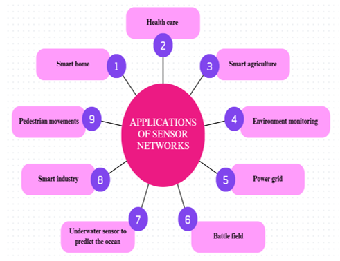
Wireless sensor networks (WSNs) are made up of individual geographically dispersed sensors that collect data in real time, alert users to events, and continuously monitor specific areas. The current research aims to find optimal algorithms to enhance network performance [1-3]. Some methods are employed to find out the shortest path [4, 5]. Routing is challenging in practical and dynamic contexts, making it one of the major issues in all applications. In this regard, routing was simulated using a genetic algorithm (GA) and fuzzy logic. Nodes have a unique ID that is evenly distributed, and the base station has a fixed position. Initially, the energy consumption of the WSN node and the data transmission distance travelled will be calculated. The fluorescence intensities are related to a function value that is stronger than glowworm brightness. Consequently, transmitting data directly to the base station results in higher power consumption, as power consumption is directly proportional to the transmission distance. Furthermore, data transmission fails when a node dies, and neighboring nodes that are unaware of the failure will continue attempting transmission, thereby wasting energy. Sensor node failures often prevent many applications from completing their data transmission processes. Fault tolerance refers to the network's ability to maintain data transfer when a node fails. Since few algorithms have been created to address fault tolerance issues, the required level of fault tolerance varies by application—for instance, a sensor used in home automation has a lower fault tolerance requirement than one used in military applications. Therefore, the application decides what level of fault tolerance is needed and various applications are shown in Figure 1. Sensor deployment consists of two phases: pre- and post-deployment. Prior to the sensor being deployed, the node structure is established during the pre-phase. In the post-deployment phase, the sensor location is established after deployment.
Figure 1. Applications of wireless sensor networks (WSNs)
In WSNs, multi-hop transmission is often employed to reduce high power dissipation over long distances. However, this approach can lead to energy imbalance, causing the network to fail prematurely [6]. To address this, the network manager can use Q-learning to construct the routing graph, thereby balancing latency and extending network lifetime. Consequently, this study aims to develop a highly reliable and lightweight data aggregation and routing protocol for next-generation IoT-integrated WSNs. The power-of-hole issue is resolved by the suggested LSDAR protocol, which divides network nodes into variable-sized clusters according to the distance calculation from the sink node. Additionally, by incorporating the best weighting functions into routing decisions, LSDAR creates routing trees using the heuristic A-star algorithm. Additionally, only a portion of the optimal tree edges are updated by monitoring the states of nodes and networks [7]. The jellyfish routing algorithm technique provides dynamic routing to increase the performance of the network [8]. The multi-hop routing protocol uses a chaotic GA that enhances the lifetime of the sensor using inter- and intra- cluster communication. The path is identified by the node and cluster head having the same identification; the gene shows the path of the next node. Based on the fitness value, the next set of nodes is generated. By this lifetime of the node, energy for individual nodes is balanced [9]. The section-based routing protocol and experimental results show that it increases the stability period by 55.88% and prolongs the lifespan of healthy nodes. The hybrid clustering routing protocol (HCP) was also used [10, 11]. Optimizing energy and routing are still important and key issues in WSNs and have been solved by clustering, bio-inspired optimization, and redesigning the protocols. In addition, swarm and evolutionary algorithms like artificial bee colony and shuffled frog leaping optimize the formation of clusters and QoS routing, and region-based and clustering-based routing protocols prolong the lifetime of the network by means of energy conservation. The scalability and energy efficiency of cluster-based schemes in node mobility and selfish node behaviour are addressed by game-theoretic approaches to promote cooperation. But little works these issues simultaneously on energy-optimization of routing, clustering, and node cooperation, motivating the current research [12-17]. A switch for data transfer was utilized for cluster heads receiving signals from nodes and for cluster head data transmission to the sink. The approach was regulated by including a threshold value in each node.
Among a group of nodes, the Butterfly Optimization Algorithm was employed to choose the optimal cluster head. The leader of the group node is elected based on parameters such as the number of nodes within a particular distance, the center of the node, current energy and distance to the base station. Chemical substances deposited on the route help to search for the path to reach the destination [18-21]. The wolf algorithm is another meta-heuristic algorithm that offers an enhanced version of the grey wolf method, which has been used to optimize network lifespan. The group formation and electing the leader of the group are done by the grey wolf algorithm [22, 23]. The grid-based reliable multi-hop routing protocol combines an optimal solution that can optimize the cluster head election process while taking data forwarding delay and reliable transmission into account.
The current work aims to enhance the lifespan of WSNs by combining techniques such as evolutionary algorithms, particle swarm optimization (PSO) and GA. Because energy consumption is proportional to data transmission frequency, the collection of repeated data reduces energy consumption [24-30]. Make effective use of the power usage of sensor nodes to overcome this drawback. Since sensors are non-rechargeable battery-based, they consume energy for three main reasons: path finding, data processing and communications. Recently, many efficient algorithms have been created for path planning. The general algorithmic adaptability of meta-heuristic algorithms to various optimization problems is noteworthy. Existing algorithms may exhibit lower performance than meta-heuristic algorithms in solving complex optimization problems due to their limited ability to adapt to diverse problem characteristics. To solve the above-mentioned issues with awareness, we used meta-heuristic algorithms like PSO, grey wolf optimization (GWO), bat algorithm (BA), etc. Therefore, it has been imperative to work over the past year to develop a path-planning routing system. In this paper, we propose a hybrid meta-heuristic algorithm to improve the drawbacks faced by sensor nodes. The goal of hybridization is to reduce any significant drawbacks while simultaneously combining the benefits of each algorithm to create a hybrid algorithm. Hybridization generally yields results that can be improved in terms of accuracy or computational speed. The initial energy for each sensor is the same for all nodes. The features of each routing protocol include path-finding, reliability, scalability, etc.
The proposed method divides the network into three types of sensor nodes, assigning specific roles for sensing, data transmission, processing, and reception. This division distributes the workload among different nodes, reduces the burden on individual sensors, and improves energy efficiency and network lifetime. Otherwise, the nodes will die prematurely. Here, we propose three types of sensors: 1. Tx/Rx sensor; 2. normal sensor; 3. aggregate sensor. The path-finding is done using a natural method called bat-finding prey. The BA finds the best route to reach the nearby base stations. To further enhance the energy of each sensor node, consider the following example: sensor s1 transmits the data along the path [s2, s6, s9] to reach the base station, and again, if sensor s1 wants to transmit the data, then the data will travel in the same direction as [s2, s6, s9]. By doing so, the energy will drain soon. Therefore, to balance the issue, we need to find out the number of iterations of data transmission. Based on the analysis, the computation of iterations is done by the ant colony algorithm. The iterations are calculated using an artificial pheromone deposited in the regular path. In Step 4, when the number of iterations exceeds the threshold value, the data is divided equally and transmitted in two directions.
2.1 Water flow algorithm
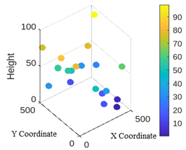
The suggested algorithm starts with fundamental processes such as a strong water flow striking a mud surface, water splitting, merging, and finally settling down when the water flow is decreased. The natural evolution rule serves as the foundation for evolutionary algorithms. The pressure is estimated from one spot to another. The water travels through small particles like stones and mud, but once it crosses a number of iterations, the path is cleared to reach the destination in a short period. While the current topology does not support scalability or network restoration, the water flow method aids in the creation of the artificial topology network. Using the pressure flow formula, a node will be created in each iteration of the water flow to move the water from one side to the other. Here, water flow is thought of as an iteration; it covers a certain area as it moves from high to low space. In the combat field application, a dynamic network link is crucial for extending the network's lifespan. The topology creation and node elevations are displayed in Figures 2 and 3, respectively.
|
Algorithm 1. Water flow algorithm (WFA) topology construction with connectivity |
|
G ← RunWaterFlowAlgorithm(V, θ) 2: connected ← CheckConnectivity(G) 3: r ← 0 4: WHILE connected = FALSE AND r < R_max DO 5: G ← AddMinimumDistanceEdges(G) 6: connected ← CheckConnectivity(G) 7: IF connected = FALSE THEN 8: θ ← UpdateParameters(θ) 9: G ← RunWaterFlowAlgorithm(V, θ) 10: connected ← CheckConnectivity(G) 11: END IF 12: r ← r + 1 13: END WHILE 14: IF connected = TRUE THEN 15: RETURN G 16: ELSE 17: RETURN FAILURE 18: END IF |
In the algorithm, V is the sensor-node set; E is the edge set; G is the graph; θ is the WFA parameter set; connected is a Boolean connectivity flag; r is the repair-attempt counter; and R_max is the maximum number of repair attempts. Function names and Boolean keywords are upright text; mathematical variables are italicized in the manuscript typesetting.
Figure 2. Nodes with elevations
Figure 3. Mathematical design and network link generation based on the water flow algorithm (WFA) topology
The starting flow is initialized with the basic parameters: iteration limit N, initial mass M, velocity Y and the limit of sub-flow, as Table 1 describes the mapping of WFA variables to WSNs.
Table 1. Mapping of water flow algorithm (WFA) variables to wireless sensor networks (WSNs) topology parameters
|
Water Flow Analogy |
Symbol |
WSN Parameter |
|
Water flow/pipe |
N, i |
Deployment paths in the target field |
|
Flow velocity |
Y |
Node deployment rate |
|
Pressure at points 1 and 2 |
l2, l1 |
Node density requirement |
|
Height at points 1 and 2 |
h2, h1 |
Elevation or terrain variation between deployment points |
|
Fluid density |
ρ |
Deployment area constraint |
|
Cross-sectional area of pipe |
A |
Communication range of a node |
|
Coverage area |
r |
Effective sensing or communication coverage radius achieved by the generated topology |
Assume N is the number of water flows in the pipe in the current iteration; it is assigned as i = {1, 2, 3, …, N}.
$n=\min \left\{\max \left\{1, \operatorname{int}\left(\frac{M_i Y_i}{T}\right)\right\}\right\}$ (1)
where, T is the time.
$Y_2=\sqrt{\frac{2\left(l_2-l_1\right)}{\rho}+Y_1^2+2 g\left(h_2-h_1\right)}$ (2)
where, l2, l1 are the pressures at points 1 and 2; g is gravity; h2, h1 are the heights at points 1 and 2; and ρ is fluid density.
$Y_i=\sqrt{Y_i^2+\frac{2 g h}{A}}$ (3)
Formula to calculate the coverage area of water as:
$r=\frac{A_{\text {pipe}} \times Y^2}{g}$ (4)
where, A is the cross-sectional area of the pipe, g is acceleration, and Y is velocity.
|
Algorithm 2. Pseudocode for the proposed optimization framework |
|
Input: N sensor nodes, base station Output: Load-balanced routing path 1. Generate artificial topology using water flow algorithm (WFA) Deploy N sensor nodes Update node positions according to water flow rules Construct topology G(V,E) 2. Apply bat algorithm (BA) for Sensor Role Assignment Initialize bat population For each sensor node Si Calculate fitness Fi based on: - Residual Energy (Ei) - Distance to base station (Di) - Node Degree (Ni) - Link Quality (Li) End For Update bat velocity and position Evaluate fitness and assign roles If Fi ≥ Flag Si ← Aggregator Sensor Else If Ftx ≤ Fi < Fagg Si ← TX/RX Sensor Else Si ← Normal Sensor End If 3. Data Collection Phase Normal Sensors → Aggregator Sensors Aggregator Sensors aggregate sensed data 4. Data Forwarding Phase Aggregator Sensors forward aggregated data through TX/RX Sensors toward the base station 5. Apply ant colony optimization (ACO) Initialize pheromone trails τij For each ant Select next hop using pheromone and heuristic information Construct route from Aggregator Sensor to base station End For Update pheromone trails Identify frequently used optimal paths 6. Load Balancing Distribute traffic among high-quality alternative routes Prevent excessive energy depletion of heavily used nodes 7. Deliver aggregated data to the base station End |
2.2 Bat algorithm
The node separation process is completed by meta-heuristic algorithms and they will guide the search process by nature and are used as one of the important techniques to solve many composite optimization problems. Among many nature-inspired algorithms, the BA is one of the algorithms introduced by Yang [31]. Because microbats are small to medium-sized bats that feed on insects, the BA is based on the echolocation behavior of microbats. It uses sonar, called echolocation, to detect prey. For example, if one microbat produces a high-pitched sound and it bounces back, it can determine the distance to prey and also the size. So the distance is measured using the following parameters: frequency, pulse rate, loudness, and position of each bat. The expression to calculate all the parameters is given below:
Step 1:
$p_i=p_{\text {min}}+\left(p_{\text {max}}-p_{\text {min}}\right)$ (5)
where, pi is the bat frequency value, pmax is the maximum frequency, and pmin is the minimum frequency. The bat will automatically adjust the frequency and frequency value depending on the size of the area.
Step 2:
$y_i^t=y_i^{t-1}\left(y_i^t-x_{\text {gbest}}^t\right) y_i$ (6)
Step 3:
$z_i^t=z_i^{t-1}+y_i^t$ (7)
where, $y_i^t$, $z_i^t$ velocity and location of the i-th bat at the period of time t.
Step 4:
$l_i^{t+1}=\alpha l_i^t$ (8)
Step 5:
$r_i^t=r_i^0\left[1-e^{-\gamma t}\right]$ (9)
where, $l_i^{t+1}$, $r_i^t$ denotes loudness and the pulse rate at the time.
2.3 Enhanced bat algorithm
An artificial bat moving in a certain direction finds the optimum answer; nevertheless, the bat's speed has a significant impact on the algorithm's accuracy and rate of convergence. Here, we are going to combine local and global search; initially, by having a higher speed, we can find the optimal solution, and at a lower speed, we can find the local solution. Based on the above analysis, the equation has been refined to solve an early problem that occurred in the basic algorithm.
Step 1
The velocity update formula:
$y_i^t=s y_i^{t-1}+\left(\left|x_i-x_j\right|+\left|y_i-y_j\right|-x_{\text {gbest}}^t\right) y_i$ (10)
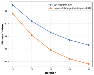
By selecting the optimal sound from among the other artificial bats, the updated formula for determining the ideal position is furthered. The random walk probability distribution function is the optimal position that was determined with the use of the Levy Fly method. By substituting the Levy flight for local searching for a single bat's ideal position, the global search process is able to produce more matching and optimization iterations, which enhances both the algorithm's convergence and accuracy. Comparative evaluation of the improved BA against baseline algorithms is illustrated in Table 2, while Figure 4 presents the corresponding convergence comparison between the standard BA and the improved BA over iterations.
Table 2. Comparative evaluation for improved bat algorithm (BA)
|
Iteration |
BA (Fitness Value) |
Improved BA (Fitness Value) |
|
10 |
0.85 |
0.78 |
|
20 |
0.72 |
0.61 |
|
30 |
0.63 |
0.49 |
|
40 |
0.57 |
0.42 |
|
50 |
0.53 |
0.38 |
Step 2
Position update equation:
$\mu=L_b+(1-c f)\left(\frac{L_b}{U_b}\right)+\left(1-\frac{\operatorname{Min}_{\text {iter}}}{\operatorname{Max}_{\text {iter}}}\right)$ (11)
$z^{i+t}=z^t \bigotimes l(\mu)$ (12)
where, Lb and Ub represent the lower bound and upper bound of frequency, and cf denotes a constant factor.
2.4 Fitness function
The proposed work requires the shortest path to reach the base station, so here the objective function is considered as distance. In this work, an artificial topology network is assigned, which further helps to search for a local optimum. The random value (rv) is initialized to a large value. By allowing the bats to move at random, it improves the algorithm's capacity for exploration and enables it to more fully explore the search space. When the iterative process comes to a conclusion, the value of wi drops, which narrows the search region surrounding the optimal solution and improves the algorithm's exploitation potential. The distance is calculated using the following formula;
$d_k=r+\frac{U b-L b}{n} * r v$ (13)
Fitness function $=\sum_{k=1}^3 \frac{d_k}{3}$ (14)
where, r is the radius of the network, n is the number of waves and rv is the random vector.
When dk is divided by 3, we can find the nearest artificial bat value. Using the above equation, we need to select the Tx/Rx among the deployed sensors and sensor nodes located at shorter distances are selected as Tx/Rx nodes, while nodes located farther away from the Tx/Rx nodes are designated as aggregator nodes based on the predefined distance criteria. Usually, a WSN is considered a group of sensor nodes. The nodes are deployed randomly. Consider a WSN with n nodes (where i = 1, 2, 3, …, n). Among these nodes, a set of Tx/Rx nodes is selected based on Eq. (1) and is responsible for data transmission. When choosing Tx/Rx, factors such as energy and node distance among the nodes are also taken into account. By considering the net optimal solution, we assume it is an aggregator node, and the rest of the nodes are considered normal nodes.
There is a requirement for data processing techniques or methodologies because the sensed data must be processed effectively to increase network performance. Hence, transmitting a larger amount of data to the base station requires more energy. Eliminating duplicate data is an aggregation technique used in WSNs that helps them use less energy. The aggregator sensor collects the data from a nearby node, aggregates the data by removing the replicated data, and finally transmits unique data to the Tx/Rx node. Every aggregation point compresses redundant data. When multiple packets are merged into a single packet using data loss aggregation, the quantity of data that is sent out is often less than what was received. When energy conservation is required and the communication load is beyond the system's capacity, this method can be helpful. When a sensor node receives duplicate copies of the same data, it has two options for processing the information: it can treat the data as duplicate and process each copy separately, or it can treat the data as one copy. The way these two functions vary is because aggregation only yields a single representative value—such as MIN, MAX, or MEDIAN—out of all the values in the dataset.
Steps for data aggregation:
Step 1: Collecting data from nearby sensors.
Step 2: Removing redundant data and sending only useful information to the Tx/Rx sensor.
Step 3: Calculating the amount of data transmitted.
The Tx/Rx sensor will collect all the data from the aggregator sensor and transmit it to the next Tx/Rx sensor.
$E_{t x}=k E_{\text {elec}}+E_{\text {amp}} d^2$ (15)
$E_{r x}=K E_{\text {elec}}$ (16)
where, Eelec represents the electronics energy, Eamp represents amplifier energy, k is bits and d is meters. Total energy consumed by this node E = Etx + Erx.
2.5 Calculation of route cost using ant colony
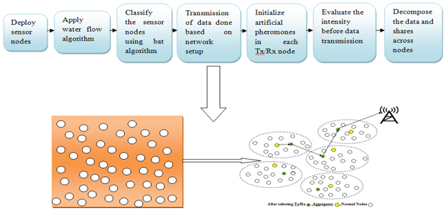
Following the conclusion of phase 1, nodes begin transmitting data from one Tx/Rx node to another. The travel cost between the nodes needs to be calculated for each iteration. The ant colony algorithm is used to compute the path cost. The ant finds the path based on semiochemicals, which are secreted by the ants themselves. The first ant starts travelling and will drop chemical substances on the ground; subsequently, another ant follows the same path. Consider the following example: The following list of ants (S1, S2, S3, S4, and S5) will find the food. Each ant goes in a different direction, and each lays a trail of pheromone where it goes. Using the meta-heuristic algorithm, each ant completes an iteration. The final ant chooses the path where it finds the highest pheromone levels. Figure 5 illustrates the overall architecture of the proposed work.
Figure 5. Architecture diagram for the proposed work
Generally, if the sensor (S1) transmits the data using the same path again and again, then the particular set of sensors will lose their energy soon compared to other sensors. The measurement has been made using the pheromone intensity value. In the optimized BA and ant colony algorithm, path planning has been done, and here we need to initialize the artificial pheromone value for all the Tx and Rx nodes. The trail from the Tx/Rx node i to the next Tx/Rx node j is created by an artificial ant placed in each Tx/Rx. Once the transmission is completed, the level of pheromone is updated on both, depending on the formula:
$\Delta \mu_{i j}=\sum_{k=0}^n \Delta \mu_{i j}$ (17)
$\mu_{i j}=(1-\alpha) \mu_{i j}+\Delta \mu_{i j}$ (18)
The route cost is calculated in the given equation.
$C=d T_x / R_{x i}-T_x / R_{x j}+\Delta \mu_{i j}$ (19)
The overall fitness functions can be expressed as follows:
$\begin{gathered}F=w_1 \frac{E_{\text {cons}}}{E_{\max}}+w_2 \frac{D_{\text {path}}}{D_{\max}}+w_3-\frac{E_{\text {res}}}{E_{\text {init}}}+w_4 \frac{\text { Delay }}{\text { Delay}_{\text {max}}}+w_5 \frac{1}{\text { Lifetime}}\end{gathered}$ (20)
where, $E_{\text {cons}}=$ total energy consumption, $D_{\text {path}}=$ routing path distance, $E_{\text {res}}=$ residual energy, $E_{\text {init}}=$ initial energy, Delay = end-to-end delay, Lifetime = network lifetime, and $w_1 w_2 w_3 w_4 w_5$ = weighting coefficients.
2.6 Data decomposition
In this section, the sensor nodes divide the original data into separate shares that are placed into a sub-array using a Vandermonde matrix [32]. Subsequently, in order to improve the reliability of perceived data transmission in WSNs, the sensor networks are utilized to send these data shares appropriately to the source node and attempt to pre-process the perceived original data using a matrix decomposition algorithm. The information that was first interpreted is expanded upon and divided into many information exchanges.
Convert these Z1 bits to Z2 y-ary digits using the following equation: Z1 = Z2 · log2y, where y represents the number of data elements.
Step 1: A = {a1, a2, ..., ad} is the result of dividing A into d vectors. Each vector can be expressed as ad={ad,1, ad,2, …, ad,m}, where m represents the number of y-ary digits contained in each subarray.
Step 2: Build an m × n y-ary Vandermonde matrix B using the set of indices b1, b2,..., and bn.
Step 3: According to Steps 1 and 2, the total number of data will be divided into n subparts, each of which is represented as a y-ary sub-array tk·td = [ad,1, ad,2, ad,3, …, ad,m], where tk = [tk,1, tk,2, tk,3, …, tk,n] includes n q-ary digits, and the symbol “·” denotes the multiplication operator in the q-ary notational system.
The Vandermonde matrix decomposition is executed at the Tx/Rx, which possesses greater computational capability than individual sensor nodes. Therefore, the additional computational cost does not increase the energy consumption of ordinary sensor nodes. The primary effect is a reduction in communication overhead through smaller or less redundant transmissions.
Since the proposed water flow algorithm (WFA), Improved BA, and ant colony optimization (ACO) algorithms are stochastic in nature, each simulation scenario was executed 30 independent times using different random seeds. The reported results correspond to the mean and standard deviation of the obtained performance metrics.
mean $=\frac{1}{n} \sum_{i=0}^n x_i$ (21)
where, $x_i$ is the performance metric obtained in the ith run; n is the total number of independent runs.
standard deviation $=\sqrt{\frac{1}{n-1} \sum_{i=1}^n\left(x_i- mean\right)^2}$ (22)
To account for the stochastic behavior of the proposed heuristic optimization framework, each simulation scenario was executed 30 independent times using different random seeds. Each simulation scenario was executed for a fixed set of network parameters, and the results reported in this study represent the performance obtained under these configurations for each corresponding network size.
2.7 Computational complexity analysis
Since the modules are executed sequentially, the overall complexity is:
$T_{\text {total}}=O\left(Q_w N+Q_b B N+Q_a A N+N\right)$ (23)
where, B represents the number of bat-algorithm agents or bats, A represents the number of ant-colony agents or ants, N the number of sensor nodes, $Q_w$ number of water flow iterations, $Q_b$ number of bat iterations, and $Q_a$ number of ant colony iterations. The simulation parameters used in this study are summarized in Table 3.
Table 3. Parameters used in MATLAB simulation
|
Number of Nodes |
50, 100, 150, 200 |
|
Distance between each node |
70 m–100 m |
|
Deployment Area |
300 × 300 m2 |
|
Ptx |
151 mW |
|
Prx |
279 mW |
|
Date Rate |
1 Mbps |
|
Data Size |
4096 bits |
|
Simulation Time |
70 s |
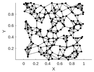
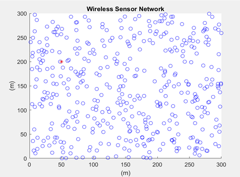
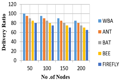
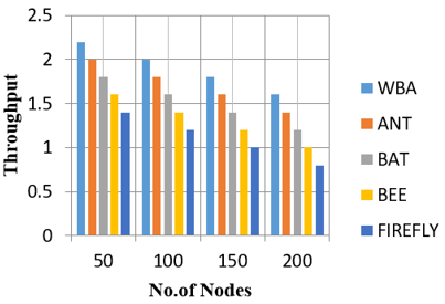
The random deployment of sensor nodes in a specific area is displayed in Figure 6. The performance comparison of the proposed WBA algorithm with ANT, BAT, BEE, and Firefly algorithms at 200 nodes is presented in Table 4.
Figure 6. Sensor deployed randomly
Table 4. Performance comparison at 200 nodes
|
Algorithm |
Delivery Ratio (%) |
Throughput |
Delay (ms) |
Network Lifetime (%) |
Energy Consumption (J) |
|
WBA |
85.2 ± 1.3 |
1.6 ± 0.05 |
10 ± 0.8 |
93 ± 1.1 |
9 ± 0.4 |
|
ANT |
80.4 ± 1.6 |
1.4 ± 0.06 |
12 ± 0.9 |
92 ± 1.3 |
11 ± 0.5 |
|
BAT |
75 ± 1.8 |
1.2 ± 0.07 |
14 ± 1.0 |
91 ± 1.4 |
13 ± 0.6 |
|
BEE |
70 ± 2.0 |
1 ± 0.08 |
16 ± 1.1 |
90 ± 1.5 |
14 ± 0.6 |
|
Firefly |
65 ± 2.2 |
0.8 ± 0.09 |
18 ± 1.2 |
89 ± 1.6 |
15 ± 0.7 |
Delivery ratio: In practical applications, the delivery ratio is a crucial statistic to take into account. While the current approach achieves a delivery ratio of 80%, the proposed work, as seen in Figure 7, yields a delivery ratio of 85%.
Figure 7. Delivery ratio versus number of nodes
Throughput: Achieving a high throughput is essential for WSNs to ensure reliable, efficient, and quick communication—a necessity for the success of numerous applications across various industries, as shown in Figure 8.
Figure 8. Throughput versus number of nodes
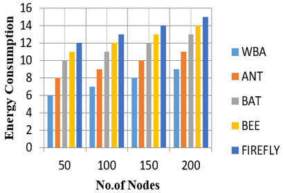
Energy consumption: Energy consumption must be managed according to the requirements of specific WSN applications to optimize network longevity and overall performance. When comparing the suggested work to the BA and ant colony algorithms, the energy consumption is 9 J, as shown in Figure 9.
Figure 9. Energy consumption versus number of nodes
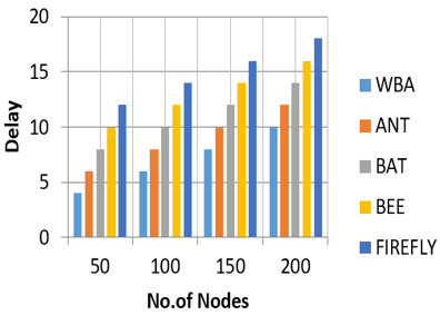
Delay: In order to provide timely and efficient communication, the network must minimize latency, especially for real-time surveillance, monitoring, and control applications. With a network size of 200, the greatest latency is 8 ms less than with the current technique represented in Figure 10.
Figure 10. Delay versus number of nodes
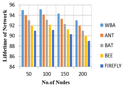
Lifetime of network: Figure 11 illustrates that the proposed WBA achieves 93% of the results, which are able to maintain a steady, effective network connection, demonstrating the importance of network lifespan in reducing data loss, improving energy efficiency, and maintaining network connectivity.
Figure 11. Lifetime of network versus number of nodes
The BA was modified by employing WFA for topology creation and by selecting the best solution among the artificial bats. The path that yields the highest number of pheromone levels is selected by the last ant. Additionally, data transmission was accomplished by dividing the data into two paths, which balanced the sensor node's energy usage. The primary goal of determining the optimal route to arrive at the destination is accomplished. WSN requires power for processing, routing, and sending bigger packets. The larger packet has been divided and sent in three separate directions by allocating the task to three distinct sensors. Sound wave path discovery increases node endurance and extends node survival for additional rounds. Further study opportunities are made possible by the extension of this approach to conceptualize transmission using a video sensor. Image data transmission is important for applications in surveillance systems and environmental monitoring systems. Instead of text data, wireless video sensors are a big part of better analysis in the modern world.
As part of future work, the experimental evaluation of the proposed approach will be extended to a broader range of network scenarios. Specifically, the effect of varying base station positions on routing efficiency and energy distribution across the network will be investigated, protocol performance will be evaluated under heterogeneous and dynamic traffic loads, and the impact of non-uniform initial energy levels among sensor nodes on network lifetime and delivery ratio will be analyzed. In addition, future evaluations will incorporate multiple independent simulation runs using different random seeds, enabling statistical reporting of results through mean, standard deviation, and 95% confidence intervals to further validate the robustness of the proposed approach.
[1] Akyildiz, I.F., Su, W., Sankarasubramaniam, Y., Cayirci, E. (2002). Wireless sensor networks: A survey. Computer Networks, 38(4): 393-422. https://doi.org/10.1016/S1389-1286(01)00302-4
[2] Pour, S.E., Javidan, R. (2021). A new energy aware cluster head selection for LEACH in wireless sensor networks. IET Wireless Sensor Systems, 11(1): 45-53. https://doi.org/10.1049/wss2.12007
[3] Singh, A., Nagaraju, A. (2020). Low latency and energy efficient routing-aware network coding-based data transmission in multi-hop and multi-sink WSN. Ad Hoc Networks, 107: 102182. https://doi.org/10.1016/j.adhoc.2020.102182
[4] Liu, Y., Wu, Q., Zhao, T., Tie, Y., Bai, F., Jin, M. (2019). An improved energy-efficient routing protocol for wireless sensor networks. Sensors, 19(20): 4579. https://doi.org/10.3390/s19204579
[5] Yu, X., Liu, Q., Liu, Y., et al. (2019). Uneven clustering routing algorithm based on glowworm swarm optimization. Ad Hoc Networks, 93: 101923. https://doi.org/10.1016/j.adhoc.2019.101923
[6] Künzel, G., Cainelli, G.P., Müller, I., Pereira, C.E. (2018). Weight adjustments in a routing algorithm for wireless sensor and actuator networks using Q-Learning. IFAC-PapersOnLine, 51(10): 58-63. https://doi.org/10.1016/j.ifacol.2018.06.236
[7] Haseeb, K., Islam, N., Saba, T., et al. (2020). LSDAR: A light-weight structure based data aggregation routing protocol with secure Internet of Things integrated next-generation sensor networks. Sustainable Cities and Society, 54: 101995. https://doi.org/10.1016/j.scs.2019.101995
[8] Christopher, V.B., Jasper, J. (2021). Jellyfish dynamic routing protocol with mobile sink for location privacy and congestion avoidance in wireless sensor networks. Journal of Systems Architecture, 112: 101840. https://doi.org/10.1016/j.sysarc.2020.101840
[9] Wang, C.H., Liu, X.L., Hu, H.S., Han, Y.J., Yao, M.Q. (2020). Energy-efficient and load-balanced clustering routing protocol for wireless sensor networks using a chaotic genetic algorithm. IEEE Access, 8: 158082-158096. https://doi.org/10.1109/ACCESS.2020.3020158
[10] Zheng, J.W., Tang, J.M., Zhou, X. (2020). Research on state multicast routing algorithm based on distributed sensing network. Procedia Computer Science, 166: 443-447. https://doi.org/10.1016/j.procs.2020.02.067
[11] Masoud, M.Z., Jaradat, Y., Zaidan, D., Jannoud, I. (2019). To cluster or not to cluster: A hybrid clustering protocol for WSN. In 2019 IEEE Jordan International Joint Conference on Electrical Engineering and Information Technology (JEEIT), Amman, Jordan, pp. 678-682. https://doi.org/10.1109/JEEIT.2019.8717524
[12] Yadav, A.S., Khushboob, K., Singha, V.K., Kushwaha, D.S. (2020). Increasing efficiency of sensor nodes by clustering in section based hybrid routing protocol with artificial bee colony. In Third International Conference on Computing and Network Communications (CoCoNet'19), 171: 887-896. https://doi.org/10.1016/j.procs.2020.04.096
[13] Dwivedi, B., Patro, B.D.K. (2019). An efficient routing algorithm for handling selfish behavior of nodes in WSN's: By using prisoner's dilemma problem. In 2019 4th International Conference on Information Systems and Computer Networks (ISCON), Mathura, India, pp. 738-741. https://doi.org/10.1109/ISCON47742.2019.9036222
[14] Zhou, J., Yang, R., Xu, M.Y. (2020). Adaptive chaotic shuffled frog leaping algorithm for QoS routing in wireless image sensor networks. In 2020 IEEE 5th International Conference on Image, Vision and Computing (ICIVC), Beijing, China, pp. 287-291. https://doi.org/10.1109/ICIVC50857.2020.9177466
[15] Xu, C., Xiong, Z.Y., Zhao, G.F., Yu, S. (2019). An energy-efficient region source routing protocol for lifetime maximization in WSN. IEEE Access, 7: 135277-135289. https://doi.org/10.1109/ACCESS.2019.2942321
[16] Sivasakthiselvan, S., Nagarajan, V. (2020). Cluster based routing schemes in mobile sensor networks: A review. In 2020 International Conference on Communication and Signal Processing (ICCSP), Chennai, India, pp. 1649-1653. https://doi.org/10.1109/ICCSP48568.2020.9182086
[17] He, W. (2019). Energy-saving algorithm and simulation of wireless sensor networks based on clustering routing protocol. IEEE Access, 7: 172505-172514. https://doi.org/10.1109/ACCESS.2019.2956068
[18] Liu, X. (2017). Routing protocols based on ant colony optimization in wireless sensor networks: A survey. IEEE Access, 5: 26303-26317. https://doi.org/10.1109/ACCESS.2017.2769663
[19] Wang, Z., Ding, H., Li, B., et al. (2020). An energy efficient routing protocol based on improved artificial bee colony algorithm for wireless sensor networks. IEEE Access, 8: 133577-133596. https://doi.org/10.1109/ACCESS.2020.3010313
[20] Maheshwari, P., Sharma, A.K., Verma, K. (2021). Energy efficient cluster based routing protocol for WSN using butterfly optimization algorithm and ant colony optimization. Ad Hoc Networks, 110: 102317. https://doi.org/10.1016/j.adhoc.2020.102317
[21] Wang, M., Wang, S., Zhang, B. (2020). APTEEN routing protocol optimization in wireless sensor networks based on combination of genetic algorithms and fruit fly optimization algorithm. Ad Hoc Networks, 102: 102138. https://doi.org/10.1016/j.adhoc.2020.102138
[22] Bhola, J., Soni, S., Cheema, G.K. (2020). Genetic algorithm based optimized leach protocol for energy efficient wireless sensor networks. Journal of Ambient Intelligence and Humanized Computing, 11: 1281-1288. https://doi.org/10.1007/s12652-019-01382-3
[23] Zivkovic, M., Bacanin, N., Zivkovic, T., Strumberger, I., Tuba, E., Tuba, M. (2020). Enhanced grey wolf algorithm for energy efficient wireless sensor networks. In 2020 Zooming Innovation in Consumer Technologies Conference (ZINC), Novi Sad, Serbia, pp. 87-92. https://doi.org/10.1109/ZINC50678.2020.9161788
[24] Chen, Z., Shen, H. (2018). A grid-based reliable multi-hop routing protocol for energy-efficient wireless sensor networks. International Journal of Distributed Sensor Networks, 14(3): 1550147718765962. https://doi.org/10.1177/1550147718765962
[25] Mohammed, L.A., Hasan, A.M., Hamza, E.K. (2024). Optimizing energy efficiency in wireless sensor networks using Dijkstra's algorithm. Instrumentation Mesure Métrologie, 23(4): 307-316. https://doi.org/10.18280/i2m.230406
[26] Zhang, J., Lin, Z., Tsai, P.W., Xu, L. (2020). Entropy-driven data aggregation method for energy-efficient wireless sensor networks. Information Fusion, 56: 103-113. https://doi.org/10.1016/j.inffus.2019.10.008
[27] Prakash, V., Pandey, S. (2023). Metaheuristic algorithm for energy efficient clustering scheme in wireless sensor networks. Microprocessors and Microsystems, 101: 104898. https://doi.org/10.1016/j.micpro.2023.104898
[28] Regilan, S., Hema, L.K. (2024). Optimizing energy efficiency and routing in wireless sensor networks through genetic algorithm-based cluster head selection in a grid-based topology. Journal of High Speed Networks, 30(4): 569-582. https://doi.org/10.3233/JHS-230209
[29] Rajaram, V., Kumaratharan, N. (2020). An optimized clustering using hybrid meta-heuristic approach for wireless sensor networks. International Journal of Communication Systems, 33(18): e4638. https://doi.org/10.1002/dac.4638
[30] Kaviarasan, S., Srinivasan, R. (2024). Developing a novel energy efficient routing protocol in WSN using adaptive remora optimization algorithm. Expert Systems with Applications, 244: 122873. https://doi.org/10.1016/j.eswa.2023.122873
[31] Yang, X.S. (2010). A new metaheuristic bat-inspired algorithm. In Nature Inspired Cooperative Strategies for Optimization (NICSO 2010), Heidelberg: Springer, pp. 65-74. https://doi.org/10.1007/978-3-642-12538-6_6
[32] Li, F., Zhou, G., Lei, J. (2019). Reliable data transmission in wireless sensor networks with data decomposition and ensemble recovery. Mathematical Biosciences and Engineering, 16(5): 4526-4545. https://doi.org/10.3934/mbe.2019226