
Hemanth Karnati | Anuraag Soma | Adnan Alam | Kalaavathi Buvaneshwaran*
© 2026 The authors. This article is published by IIETA and is licensed under the CC BY 4.0 license (http://creativecommons.org/licenses/by/4.0/).
OPEN ACCESS
Low-cost gas, particulate and climatic sensors enable dense, real-time indoor air quality (IAQ) monitoring, but their outputs are sensor-specific indices rather than regulatory-grade measurements: MQ7 is mainly CO-sensitive, MQ135 is a broad “air-quality” gas sensor, rather than a quantitative nitrogen oxides (NOₓ) instrument, CCS811 reports algorithm-derived equivalent CO₂ (eCO₂) and total volatile organic compound (TVOC) estimates, and GP2Y1010 yields a dust proxy rather than a standard PM₂.₅/PM₁₀ reading. This pilot study presents a low-cost monitoring stack (Arduino Uno + ESP8266 + the five sensors above) with a documented per-sensor calibration framework, an explicit uncertainty budget propagated to the observed between-environment differences, and a transparent disclosure of which conversions were actually applied to the recorded data. Two paired 24 h deployments (6 April 2024 for the indoor room and 5 May 2024 for the kitchen) were logged via ThingSpeak in a regular indoor room (1,333 samples; median sampling interval 62 s) and in a hostel-mess kitchen with overhead exhaust hoods and air blowers (1,253 samples; median interval 45 s). Across the kitchen samples, TVOC exceeded 300 ppb for approximately 7.7 h (32% of the deployment) and eCO₂ exceeded 1,000 ppm for approximately 15.3 h (64% of the deployment). The kitchen TVOC peak of approximately 3,862 ppb exceeds the CCS811 data-sheet ceiling of 1,187 ppb; the 300 ppb threshold was therefore used for cooking-window separation. These observations are consistent with the hypothesis that conventional exhaust ventilation may only partially mitigate cooking emissions at occupant distance under the observed operating conditions; they are not a confirmatory population-level claim. Raw data are publicly released, while firmware and the analysis pipeline are available on request.
indoor air quality, low-cost sensors, sensor calibration and uncertainty, cross-sensitivity, IoT, CCS811, MQ-series, kitchen ventilation
Indoor air quality (IAQ) has increasingly become a focus of environmental health research due to its critical implications for human health. Cooking-related activities, in particular, are significant contributors to indoor air pollution, especially in environments such as kitchens in hostel messes. This pollution comprises various hazardous substances, including volatile organic compounds (VOCs), carbon monoxide (CO), nitrogen oxides (NOₓ), and particulate matter [1, 2]; exposure to indoor VOCs in particular has long been linked to sensory irritation and adverse comfort and health outcomes [3]. The World Health Organization has highlighted the severity of household air pollution, attributing approximately 3.2 million premature deaths annually to it [4].
Despite the proliferation of IoT-based IAQ monitoring systems, two related gaps remain. First, low-cost sensors are typically not metrologically calibrated against reference instruments, so their outputs should be treated as sensor-specific indices rather than regulatory-grade concentrations [5, 6]. Second, most field studies report descriptive statistics without documenting sampling intervals, missing-data handling, or the exact reproducibility artefacts needed for independent verification. These weaknesses motivate a measurement-quality-first framing for the present work.
This study designs, deploys, and evaluates a sensor-driven IAQ monitoring system tailored for kitchen environments. The principal contribution is not a quantitative pollutant report (which would require co-located reference instruments) but rather a calibration-disclosure protocol for the low-cost-sensor stack: the data-sheet calibration framework that would be required for regulatory-grade reporting is documented in full (Section 3.3, Eqs. (1) and (2)), accompanied by an explicit, line-by-line statement of which conversions were and were not instantiated in this pilot. This documented framework is then exercised on a kitchen-versus-indoor pilot under a percentile-aware and cooking-window-aware analysis. The framework, the raw datasets, and the data dictionary are released for replication.
2.1 Low-cost sensor calibration and cross-sensitivity
Low-cost gas and particulate sensors (the MQ-series, CCS811, GP2Y1010, Bosch BME680, etc.) are widely used in IoT-based IAQ monitoring [6-9], yet they are known to require careful calibration and cross-sensitivity handling. Ródenas García et al. [10] catalogue calibration, reliability and standardisation as the principal open issues for low-cost IAQ sensors. Sá et al. [6] arrive at the same conclusion in their review of low-cost sensing technology, noting that ppm-level claims from uncalibrated sensors should be treated as relative indices. Bousiotis et al. [5] co-located four low-cost particulate sensors with research-grade instruments and found that, while the relative trends were preserved, the absolute concentrations diverged substantially. These results frame the interpretation we adopt below: relative kitchen vs. indoor comparisons are defensible; absolute regulatory-grade concentrations are not.
Beyond cataloguing these limitations, the measurement-science literature prescribes how low-cost sensors should be field-calibrated and validated. Spinelle et al. [11] show that field calibration against co-located reference analysers—rather than laboratory or data-sheet curves alone—is a prerequisite for quantitative use of low-cost gas sensors, and Maag et al. [12] survey calibration strategies across air-pollution monitoring deployments, treating offset/gain correction, sensor fusion and periodic recalibration as the principal remedies for sensor drift. Drift and calibration transfer are first-order effects: Tancev and Pascale [13] show that field-calibrated sensor systems incur a systematic sampling bias when relocated from their calibration environment, and Karagulian et al. [14] consolidate field-evaluation results across commercial low-cost sensors, reporting device-to-device performance variation large enough to make validation deployment-specific. Within instrumentation practice, De Capua et al. [15] likewise propose strategies for improving the measurement quality of IAQ monitoring systems. This literature motivates the stance adopted here: with no co-located reference instrument available, the data-sheet calibration framework is documented in full and propagated to an explicit uncertainty statement (Section 3.3), but absolute concentrations are not claimed.
2.2 Practical meaning and limitations of eCO₂ and total volatile organic compound estimates
The CCS811 and similar metal-oxide gas sensors report on-chip algorithm-derived eCO₂ and total volatile organic compound (TVOC) values from a single sensor element. These outputs are useful trend indicators but do not measure CO₂ or speciated VOCs directly. Zhu et al. [16] explicitly treat CCS811-derived eCO₂ as an indicator for forecasting purposes rather than as ground-truth CO₂; the chip baseline is known to drift in sustained high-VOC environments without clean-air exposure. Shin et al. [17] note the same caveat in their monitoring work coupled to heating, ventilation and air conditioning (HVAC) systems. The TVOC value, in particular, is a composite, un-speciated proxy whose absolute magnitude is sensitive to humidity and to the chip’s internal compensation state.
2.3 Ventilation evaluation in kitchen environments
Kitchens are an under-studied but high-exposure subset of the IAQ monitoring problem space. Cooking events release CO, VOCs, NOₓ, and particulate matter at concentrations that can exceed outdoor levels; the effectiveness of exhaust hoods and ventilation openings depends strongly on flow rate, capture geometry, and occupant distance. Existing IoT-based IAQ deployments [7, 9, 18-21] either report a single-environment study without ventilation context or evaluate office and residential settings rather than institutional kitchens [22, 23]. The present pilot adopts a kitchen-versus-room comparison as a case study for the documented calibration framework above, rather than as the principal contribution. The interpretation is bounded by the limitations stated explicitly in Section 7: no air-change-rate measurement, no exhaust on/off comparison, and a single 24 h deployment per environment.
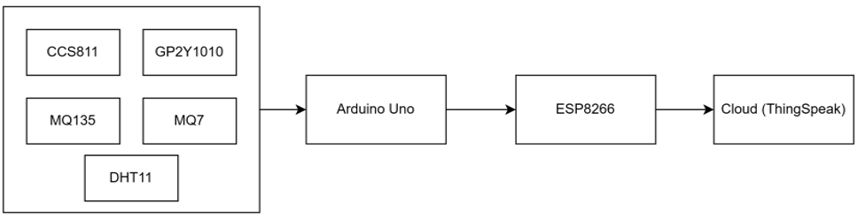
The methodology consists of a hardware stack (Section 3.1), a firmware and cloud-telemetry layer (Section 3.2), and the calibration framework and uncertainty disclosure that motivate the interpretation of the recorded values (Section 3.3). The overall system architecture is shown in Figure 1.
3.1 Hardware
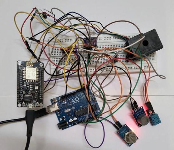
The hardware foundation comprises an Arduino Uno (central processing), an ESP8266 NodeMCU v3 (Wi-Fi cloud telemetry), and five sensors selected to span the four pollutant families relevant to kitchens (combustion gases, general AQI gases, VOC/eCO₂ and particulate matter) and the climatic covariates needed for sensor compensation. The microcontroller wiring map is given in Table 1 and the assembled prototype is shown in Figure 2.
Table 1. Microcontroller connection map for the five-sensor stack
|
Component |
Connection Type |
Connection Details |
|
DHT11 |
VCC/GND/Data |
5 V/GND/Digital Pin 2 (Arduino) |
|
MQ7 |
VCC/GND/A out/ |
5 V/GND/Analog A0 (Arduino) |
|
MQ135 |
VCC/GND/A out/ |
5 V/GND/Analog A1 (Arduino) |
|
GP2Y1010 |
VCC/GND/A out/LED |
5 V/GND/Analog A2/Digital Pin 3 (Arduino) |
|
CCS811 |
VCC/GND/SDA/SCL/WAKE |
3.3 V/GND/GPIO4/GPIO5/GND (ESP8266) |
|
UART link |
Arduino TX/RX/GND↔ESP8266 RX/TX/GND |
9,600 baud |
Figure 2. Assembled prototype: Arduino Uno, ESP8266 NodeMCU v3 and the five sensors on a single perfboard
MQ7 (Henan Hanwei) provides an analog 10-bit ADC output, which primarily reflects changes in the resistance of its tin dioxide (SnO₂) film in response to reducing gases. While the sensor is most sensitive to CO, it is also cross-sensitive to hydrogen, alcohol, and methane. Its application is limited by its non-quantitative nature for CO, as well as the requirement for preheating (>60 min) and an R₀ baseline established in clean air to derive ppm values via the data-sheet log-log curve. Because the in-situ R₀ procedure was not performed in this pilot study, the MQ7 outputs are treated as ppm-equivalent relative concentration indicators (Section 3.3).
The MQ135 (Henan Hanwei) provides an analog 10-bit ADC output that responds to a broad spectrum of pollutants (e.g., NH₃, NOₓ, alcohol, smoke, and CO₂). Therefore, its signal is treated as a general "air quality index". Key limitations include its non-selective response (it is not a quantitative NOₓ instrument) and the humidity dependence of its calibration curves. Consistent with Section 2.1, the MQ135 output is interpreted as a relative index or a ppm-equivalent value in this study.
The CCS811 (AMS/ScioSense) provides digital equivalent CO₂ (eCO₂; 400–8,192 ppm) and total volatile organic compound (TVOC; 0–1,187 ppb according to the manufacturer) values, computed by an on-chip algorithm from a single metal-oxide (MOX) element. These values serve as trend indicators rather than direct measurements of CO₂ or speciated VOCs. The sensor's specifications include ±10% manufacturer accuracy, a 20-min warm-up to a usable state, and 48 h to reach a stable baseline (all of which were honoured in this pilot). Although the on-chip ENV_DATA register accepts external temperature and relative humidity (T/RH) for compensation, the ESP8266 firmware did not populate this register, so the chip operated with its default internal compensation.
Regarding out-of-range TVOC values, the kitchen dataset (stored as a comma-separated values [CSV] file) contains TVOC samples up to approximately 3,862 ppb during the highest cooking peaks, well beyond the data-sheet ceiling of 1,187 ppb. These raw values are retained unmodified for transparency but should be interpreted as saturated, out-of-specification outputs indicating a "high-VOC episode" rather than calibrated concentrations. The cooking-window separation in Section 6.3 is therefore based on a 300 ppb threshold (well within specification) rather than on the absolute peak magnitudes. This limitation is acknowledged in Section 7.
The GP2Y1010 (Sharp) outputs an analog 10-bit ADC value from an LED-photodiode optical scatter sensor. This output serves as a dust-scattering proxy rather than a calibrated PM₂.₅ or PM₁₀ value. The sensor is not size-selective, and the datasheet linear conversion (Vₒ = K⋅ρ + Voc) requires measuring the dark-current offset (Voc), which was not performed in this pilot. Consequently, the GP2Y1010 readings are treated as a relative dust indicator.
The DHT11 (Aosong) provides digital temperature (±2 ℃) and relative humidity (±5% RH) readings, quantised to integers. These serve as ambient climatic covariates required for downstream sensor compensation. However, the sensor has low precision, with a resolution of 1 ℃ for temperature and 1% for relative humidity.
3.2 Software and cloud telemetry
The firmware was developed in the Arduino IDE (C/C++). The Arduino sketch drives the GP2Y1010 ILED pulse train (320 µs on / 9.68 ms off per the Sharp datasheet) and reads its analog output mid-pulse; it reads the MQ7, MQ135 and DHT11 channels once per cycle and ships the five Arduino-side fields over UART to the ESP8266. The ESP8266 reads the CCS811 eCO₂ and TVOC values via I²C using the SparkFun CCS811 Arduino library, concatenates the seven channels, and uploads them to ThingSpeak, following the Wi-Fi/cloud telemetry pattern that is standard in IoT-based IAQ monitoring [24]. The ThingSpeak free tier rate-limits a channel write to roughly one every 15 s; the firmware budgets one upload per sensor cycle, yielding the median sampling intervals reported in Section 4.2 (62 s indoor and 45 s kitchen). Inter-sample gaps caused by transient Wi-Fi reconnections are not imputed: missing cycles simply yield no row in the CSV. The CCS811 was given a 20-min warm-up before logging began in both environments. The on-chip ENV_DATA T/RH compensation register was not populated by the firmware in this pilot; the chip therefore ran with its default internal compensation.
3.3 Sensor calibration framework and uncertainty
A central weakness of much low-cost IAQ work is the absence of an explicit calibration disclosure. This section documents the data-sheet calibration framework that the present sensor stack would require for regulatory-grade reporting, together with an explicit statement of which conversions were and were not applied in this pilot.
MQ-series (MQ7 and MQ135). For a fully calibrated deployment, the sensor resistance Rₛ is recovered from the analog output Vₒ across the on-board load resistor Rₗ (10 kΩ) driven from VCC = 5 V:
Rₛ = Rₗ ⋅ (VCC / Vₒ − 1) (1)
The gas concentration would then be read off the data-sheet log-log curve:
log₁₀(ppm) = m ⋅ log₁₀(Rₛ/R₀) + b (2)
with sensor-specific (m, b) from the Henan Hanwei datasheets (m ≈ −0.66, b ≈ 1.10 for the MQ7 CO branch; m ≈ −0.42, b ≈ 0.86 for the MQ135 CO₂ branch). R₀ is the sensor’s baseline resistance in clean air at 20 ℃/65% RH.
What was actually applied in this pilot. No in-situ R₀ calibration was performed, no log-log conversion to ppm was applied, and the humidity/temperature compensation coefficients were not fitted. The MQ7 and MQ135 columns in the released CSV files contain the raw 10-bit Arduino ADC counts. Throughout this paper, these columns are labelled ppm-equivalent/relative concentration and are treated as relative trend indicators between the two environments, not as calibrated absolute concentrations.
CCS811. The manufacturer-stated accuracy is ±10% of reading for both eCO₂ (400–8,192 ppm) and TVOC (0–1,187 ppb). The sensor requires a 20-min warm-up to reach a usable state and 48 h to establish a stable baseline. The ENV_DATA T/RH compensation register was not populated by the firmware in this pilot; absolute eCO₂ and TVOC magnitudes are therefore chip outputs under default compensation, not co-located ground truth.
GP2Y1010. Datasheet linear scatter model Vₒ = K⋅ρ + Voc with K ≈ 0.5 V per 100 µg/m³ and Voc ≈ 0.9 V. Voc was not measured for the specific device used in this pilot; the dust column in the released CSVs is therefore the raw ADC output, treated as a relative dust indicator.
DHT11. Datasheet accuracy of ±2 ℃ and ±5% RH, with these error limits carried into the uncertainty budget presented in Table 2.
Table 2. Per-channel uncertainty budget
|
Channel |
Sensor |
Accuracy |
Resolution |
Warm-up |
|
CO-equivalent (ppm-eq) |
MQ7 |
±15% (RH-dependent) |
10-bit ADC |
>60 min |
|
AQI-equivalent (ppm-eq) |
MQ135 |
±15% (RH-dependent) |
10-bit ADC |
>60 min |
|
Temperature (℃) |
DHT11 |
±2 ℃ |
1 ℃ |
— |
|
Relative humidity (%) |
DHT11 |
±5% RH |
1% |
— |
|
eCO₂ (ppm) |
CCS811 |
±10% of reading |
1 ppm |
20-min usable / 48 h stable |
|
TVOC (ppb) |
CCS811 |
±10% of reading |
1 ppb |
20-min usable / 48 h stable |
|
Dust (sensor index) |
GP2Y1010 |
±15% (per datasheet) |
10-bit ADC |
— |
Uncertainty propagation to the observed environment differences. The accuracy bounds in Table 2 are manufacturer specifications; to make their analytical consequence explicit, they are propagated to the kitchen-versus-indoor comparison as type-B uncertainties following the GUM [25]. A fractional accuracy specification a (e.g., a = 0.10 for the CCS811 channels) is treated as a rectangular bound, giving a standard uncertainty u(x) = a·x/√3 for a reading x. For the difference Δ between the two environment means (kitchen minus indoor), the combined standard uncertainty is u(Δ) = √(u₁² + u₂²) = (a/√3)·√(x₁² + x₂²), where u₁ = a·x₁/√3 and u₂ = a·x₂/√3 are the standard uncertainties of the kitchen mean x₁ and the indoor mean x₂, under the conservative worst-case assumption that the systematic errors of the two deployments do not cancel; for the fixed DHT11 bounds b (±2 ℃, ±5% RH), u₁ = u₂ = b/√3, so that u(Δ) = √2·b/√3. Because the identical sensor node was redeployed across the two sites, a stable gain error would scale both environments similarly, so this bound overstates the uncertainty of the relative comparison; it also excludes calibration-model error, which is undefined for the uninstantiated conversions of Eqs. (1) and (2). Section 6.1 applies this propagation channel by channel and compares u(Δ) with the observed differences.
4.1 Environments and deployment
The system was deployed in two distinct environments to compare their air quality. The indoor (control) site was a standard student residential room without in-room cooking, without air conditioning, and with passive cross-ventilation through a single window. The kitchen site was a hostel-mess kitchen equipped with overhead exhaust hoods and wall-mounted air blowers, where approximately 200 meals per day are cooked on multi-burner liquefied petroleum gas (LPG) stoves; the adequacy of this ventilation under sustained cooking is the question we examine. The monitoring node was placed approximately 4.6 m (15 ft) horizontally from the nearest active burner, at a height of 1.5 m, on a stainless-steel preparation counter outside the immediate hood-capture zone.
4.2 Sampling, preprocessing and missing-value handling
Both deployments lasted approximately 24 h. The indoor deployment ran from 6 April 2024 12:00 IST to 7 April 2024 11:59 IST (1,333 samples; duration 23.99 h); the kitchen deployment ran from 5 May 2024 09:02 IST to 6 May 2024 08:50 IST (1,253 samples; duration 23.80 h). All timestamps are in Indian Standard Time (UTC + 05:30) as configured on the ThingSpeak channel. The median sampling interval was 62 s in the indoor deployment (IQR [61, 62] s) and 45 s in the kitchen deployment (IQR [42, 82] s); the wider kitchen IQR reflects occasional ESP8266 Wi-Fi reconnections. The longest single inter-sample gap was 37.0 min in the indoor deployment and 22.0 min in the kitchen deployment, in both cases attributable to transient Wi-Fi outages. The field-level CSV files contain no NaN values after the platform recorded the channel write; the analysis pipeline therefore treats inter-sample gaps as missing-by-design and performs no imputation. Hourly summary plots use a one-hour resample-by-mean window anchored at the top of each clock hour, computed via pandas DataFrame.resample('1h').mean(); all per-channel summary statistics in Section 6 operate on the raw per-sample data.
4.3 Data dictionary
Table 3 provides the data dictionary for the raw CSV files released with this study.
Table 3. Data dictionary for the released CSV files
|
Column |
Type |
Units |
Sensor |
Description |
|
created_at |
ISO-8601 timestamp |
IST (UTC + 05:30) |
— |
ThingSpeak channel-write timestamp |
|
entry_id |
integer |
— |
— |
Monotonic ThingSpeak entry counter |
|
field1 |
integer |
10-bit ADC |
MQ7 |
CO-sensitive metal-oxide gas sensor; ppm-equivalent |
|
field2 |
integer |
10-bit ADC |
MQ135 |
General AQI metal-oxide gas sensor; ppm-equivalent |
|
field3 |
integer/float |
℃ |
DHT11 |
Ambient temperature, ±2 ℃ |
|
field4 |
integer/float |
% RH |
DHT11 |
Relative humidity, ±5% |
|
field5 |
integer/float |
ppm (CCS811 algo) |
CCS811 |
On-chip eCO₂ estimate, ±10% |
|
field6 |
integer/float |
ppb (CCS811 algo) |
CCS811 |
On-chip TVOC estimate, ±10% |
|
field7 |
integer |
10-bit ADC |
GP2Y1010 |
Optical dust scatter proxy; not size-selective |
|
lat/lon/elev/status |
various |
— |
— |
ThingSpeak metadata; unused |
Per-channel summary statistics (mean, standard deviation (SD), minimum, maximum, and the 25th/50th/75th percentiles shown in Table 4; 5th and 95th percentiles available in the released CSVs) are computed on the raw per-sample data for each environment using NumPy on the released CSVs. Correlation matrices use the Pearson product-moment correlation computed on all paired non-missing per-sample values (indoor n = 1,333; kitchen n = 1,253); they are presented as exploratory descriptive summaries and correlation does not establish causation. A cooking-window separation is defined by the kitchen TVOC value at each sample: samples with TVOC > 300 ppb are labelled cooking, others non-cooking. This threshold corresponds to approximately 8× the indoor mean TVOC and exceeds the indoor 99th percentile, making it a conservative indicator of cooking-driven VOC elevation rather than a regulatory cut-off. In keeping with this descriptive framing, between-environment contrasts are additionally quantified in Section 6.1 in two complementary ways: as descriptive standardized effect sizes (Cohen’s d on the pooled per-sample SD) and as the ratio of the observed mean difference to the propagated instrument uncertainty u(Δ) of Section 3.3; neither is given an inferential interpretation, given the strong per-sample autocorrelation noted in Section 7.
Table 4. Per-channel summary statistics for the indoor and kitchen deployments
|
Channel |
Indoor Mean ± SD |
Indoor P25/P50/P75 |
Indoor Min–max |
Kitchen Mean ± SD |
Kitchen P25/P50/P75 |
Kitchen Min–max |
|
MQ7 (ppm-eq) |
185.7 ± 15.0 |
172.0/188.0/196.0 |
149.0–228.0 |
251.1 ± 56.4 |
209.0/231.0/290.0 |
176.0–417.0 |
|
MQ135 (ppm-eq) |
40.1 ± 2.8 |
38.0/40.0/42.0 |
35.0–50.0 |
39.5 ± 4.2 |
37.0/38.0/41.0 |
32.0–57.0 |
|
Temperature (℃) |
32.8 ± 1.0 |
31.8/33.3/33.7 |
30.7–34.2 |
35.5 ± 1.8 |
34.2/35.2/36.3 |
32.8–40.1 |
|
Humidity (%) |
55.4 ± 9.5 |
45.0/57.0/66.0 |
39.0–69.0 |
72.9 ± 9.5 |
65.0/77.0/81.0 |
50.0–87.0 |
|
eCO₂ (ppm) |
650.1 ± 147.3 |
548.0/615.0/715.0 |
400.0–1,518 |
1,360 ± 613.7 |
813.0/1,313/1,783 |
400.0–3,480 |
|
TVOC (ppb) |
37.6 ± 22.6 |
22.0/32.0/47.0 |
0.0–184.0 |
374.6 ± 595.4 |
62.0/139.0/431.0 |
0.0–3,862 |
|
Dust (sensor index) |
14.8 ± 72.2 |
0.0/0.0/4.0 |
0.0–625.0 |
46.8 ± 26.7 |
39.0/47.0/52.0 |
0.0–186.0 |
6.1 Per-channel summary statistics and percentiles
Table 4 reports the per-channel summary statistics for the two environments. As anticipated under the calibration disclosure of Section 3.3, absolute values for MQ7, MQ135, and the dust channel are reported as ppm-equivalent or sensor-index, not as calibrated absolute concentrations. TVOC is consistently reported in ppb and eCO₂ in ppm throughout. The kitchen distributions are visibly more heavy-tailed for the chemistry channels (TVOC, eCO₂) than the indoor distributions, as expected for episodic cooking events. The indoor dust channel is the exception: its mean (14.8) and SD (72.2) are dominated by intermittent spikes rather than by a sustained level. Sixty of the 1,333 indoor samples (4.5%) exceed 50 and contribute about 83% of the summed signal, and 29 of the 30 samples above the kitchen maximum of 186 fall in the last 70 min of the deployment (10:52–11:57 IST on 07 April 2024), where the readings alternate between zero and values of up to 625 with no accompanying change in the other channels. The released data do not identify the source of this late cluster, so the readings are retained as recorded. Excluding the samples above 50, the indoor dust mean is 2.6 (SD 5.7). These spikes therefore raise the indoor mean, which implies that the kitchen-minus-indoor dust difference reported in Table 5 is, if anything, understated; consequently, the indoor median (0.0) is a more representative summary for this channel.
To ground the comparison quantitatively, Table 5 reports the kitchen-versus-indoor mean difference Δ for each channel alongside (i) the combined standard uncertainty u(Δ) propagated from the Table 2 accuracy bounds (Section 3.3) and (ii) the descriptive standardized effect size (Cohen’s d on the pooled per-sample SD). Six of the seven channels show |Δ| / u(Δ) > 1, with the chemistry and moisture channels well clear of the instrument bound—eCO₂ (≈8×), TVOC (≈15×), dust (≈8×) and humidity (≈4×)—so the observed kitchen–indoor contrasts on these channels cannot be attributed to manufacturer accuracy specifications alone. The MQ135 difference lies well within its propagated uncertainty (|Δ| / u(Δ) ≈ 0.1) and is therefore not interpreted. The two framings are complementary: TVOC combines the largest uncertainty ratio with a moderate d (≈0.8) because its within-kitchen variance is dominated by episodic cooking peaks, whereas the climatic channels show large d with modest uncertainty ratios. All effect sizes are descriptive; no inferential claim is attached (Sections 5 and 7).
Table 5. Kitchen-versus-indoor mean differences relative to propagated instrument uncertainty and descriptive effect size
|
Channel |
Δ (Kitchen–Indoor) |
u(Δ) |
|Δ| / u(Δ) |
Cohen’s d |
|
MQ7 (ppm-eq) |
+65.4 |
27.0 |
2.4 |
1.58 |
|
MQ135 (ppm-eq) |
−0.6 |
4.9 |
0.1 |
−0.17 |
|
Temperature (℃) |
+2.7 |
1.6 |
1.7 |
1.85 |
|
Humidity (% RH) |
+17.5 |
4.1 |
4.3 |
1.84 |
|
eCO₂ (ppm) |
+709.9 |
87.0 |
8.2 |
1.59 |
|
TVOC (ppb) |
+337.0 |
21.7 |
15.5 |
0.80 |
|
Dust (sensor index) |
+32.0 |
4.3 |
7.5 |
0.59 |
6.2 Correlation structure
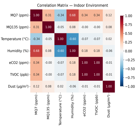
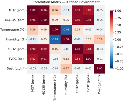
Figures 3 and 4 show the per-environment Pearson correlation matrices for the seven recorded channels. Both matrices are computed on all paired non-missing per-sample values (indoor n = 1,333; kitchen n = 1,253). These matrices are exploratory, as correlation does not establish causation. Furthermore, both matrices should be interpreted in light of the CCS811's on-chip algorithmic coupling: under quiet, low-VOC conditions, the chip's internal model drives eCO₂ and TVOC nearly deterministically from a common metal-oxide (MOX) baseline. Consequently, the very high indoor TVOC↔eCO₂ correlation reflects the on-chip algorithm rather than an atmospheric coupling. The indoor matrix accordingly shows a near-perfect TVOC↔eCO₂ correlation, together with moderate positive coupling between humidity and the MQ-series and a moderate inverse coupling between temperature and humidity.
The kitchen matrix shows the opposite pattern of interest: the TVOC↔eCO₂ correlation is lower than in the indoor matrix. This occurs because the chip's algorithmic coupling is partially broken by genuine, transient VOC injections from cooking, which the eCO₂ branch does not track in lockstep. Meanwhile, TVOC and eCO₂ both develop meaningful positive couplings with temperature and humidity, consistent with the expectation that cooking events simultaneously elevate heat, water vapour, and VOC emissions.
6.3 Cooking versus non-cooking sample separation
Under the cooking-window definition introduced in Section 5 (TVOC > 300 ppb at the per-sample level), 404 of the 1,253 kitchen samples (approximately 32%) qualify as cooking samples. Table 6 contrasts the cooking-window median with the non-cooking-window median for each kitchen channel. The TVOC and eCO₂ channels separate strongly between the two regimes (TVOC median ratio approximately 8×; eCO₂ median ratio approximately 2×), while the MQ-series and climatic channels show smaller separations.
Table 6. Kitchen samples separated by total volatile organic compound (TVOC) threshold
|
Channel |
Cooking Median |
Non-cooking Median |
Ratio |
|
MQ7 (ppm-eq) |
319 |
214 |
1.49× |
|
MQ135 (ppm-eq) |
44 |
37 |
1.19× |
|
Temperature (℃) |
34.7 |
35.2 |
0.99× |
|
Humidity (%) |
77.0 |
77.0 |
1.00× |
|
eCO₂ (ppm) |
1,948 |
964 |
2.02× |
|
TVOC (ppb) |
659 |
85 |
7.75× |
|
Dust (sensor index) |
47 |
46 |
1.02× |
Across all kitchen samples, TVOC exceeded the 300 ppb threshold for a sample-weighted total of approximately 7.7 h (32% of the deployment) and kitchen eCO₂ exceeded 1,000 ppm—a commonly cited indoor-air-quality comfort threshold—for a sample-weighted total of approximately 15.3 h (64% of the deployment). Both figures are aggregations of all samples above the threshold (each kitchen sample weighted by the deployment-mean inter-sample interval of ≈68 s, i.e., the deployment duration of 23.80 h divided by the 1,253 samples); they are not the duration of any single contiguous cooking episode. The mean interval is used for this weighting rather than the 45 s median (Section 4.2) because the total sample count multiplied by the mean interval recovers the deployment duration, whereas the median does not reflect the longer inter-sample gaps caused by Wi-Fi reconnections and would understate elapsed time. Considered together with the calibration disclosure (Section 3.3) and the limitations (Section 7), these observations are consistent with the hypothesis that conventional exhaust ventilation may only partially mitigate cooking emissions at occupant distance under the observed operating conditions, but they are not a confirmatory population-level claim.
6.4 Hourly patterns and time-series visualisation
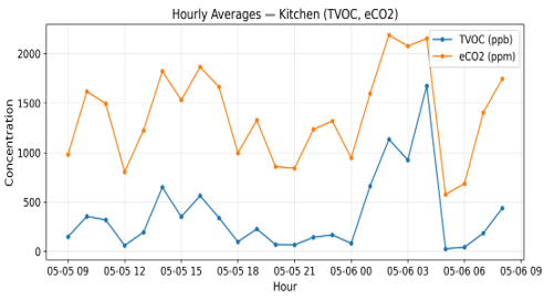
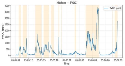
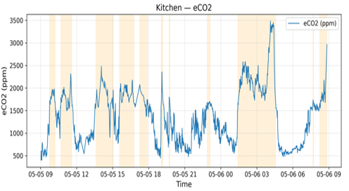
Figures 5-7 summarise the kitchen deployment at hourly and per-sample resolution. Figure 5 shows hourly-averaged TVOC and eCO₂, both peaking during the canonical lunch and dinner preparation windows.
Figure 5. Hourly-averaged kitchen total volatile organic compound (TVOC) and eCO₂ concentrations
Figure 6 shows the raw TVOC time series with cooking-window samples shaded, and Figure 7 shows the corresponding eCO₂ series, visually confirming that the TVOC and eCO₂ cooking peaks co-occur.
This pilot study has several limitations that should be acknowledged. (1) No co-located reference instrument. No reference-grade TVOC analyser, non-dispersive infrared (NDIR) CO₂ sensor, or beta-attenuation PM monitor was available; absolute CCS811 magnitudes are chip outputs under default compensation, not ground truth. (2) Calibration framework not instantiated in this pilot. MQ-series and GP2Y1010 conversions (Eqs. (1) and (2)) were not applied; values are ppm-equivalent/sensor-index; the uncertainty propagation of Sections 3.3 and 6.1 therefore covers manufacturer specification bounds only, not calibration-model error. (3) CCS811 TVOC saturation during cooking peaks. The chip’s data-sheet TVOC ceiling is 1,187 ppb; the kitchen deployment recorded values up to approximately 3,862 ppb during the strongest cooking episodes (Section 3.1). All threshold-based analysis in this paper (cooking-window separation and the 7.7 h above-threshold metric) uses a 300 ppb cut-off, which is well within the chip’s certified linear range and is therefore unaffected by saturation; the absolute peak magnitudes themselves are not interpreted quantitatively. (4) No ventilation operating-state data. No measurement of exhaust-hood flow rate, air-change rate, window position, or exhaust on/off state was recorded; the exhaust-partial-mitigation claim is limited to the observed conditions and is hypothesis-generating, not confirmatory. (5) Single 24 h deployment per environment with a calendar gap between sites (6 April vs. 5 May 2024). (6) Per-sample autocorrelation. We confine reporting to descriptive statistics (means, percentiles, medians) and exploratory Pearson correlations; we do not report null-hypothesis significance tests.
This pilot study presented a documented calibration and uncertainty framework for a low-cost air-quality monitoring stack (Arduino Uno + ESP8266 + MQ7 + MQ135 + CCS811 + GP2Y1010 + DHT11), with a transparent disclosure of the applied and unapplied conversions. The framework was applied to paired 24 h deployments in a regular indoor room and a hostel-mess kitchen, enabling a robust comparison of the two environments. Kitchen samples exhibited TVOC above 300 ppb for approximately 7.7 h (32%) and eCO₂ above 1,000 ppm for approximately 15.3 h (64%), with cooking vs. non-cooking sample medians separating strongly for TVOC and eCO₂. The dominant contrasts—eCO₂, TVOC, dust and humidity—exceeded the instrument-uncertainty bounds by factors of approximately 4–15, so the observed separations are not merely artefacts of sensor accuracy specifications. However, bounded by the calibration disclosure and the limitations discussed above—notably, the absence of co-located reference instruments and direct ventilation-operating-state measurements—these findings are consistent with the hypothesis that conventional exhaust ventilation may only partially mitigate cooking emissions at occupant distance under the observed conditions. They do not constitute a confirmatory population-level claim. Future work should involve multi-day, multi-kitchen deployments with reference co-location.
Four follow-on directions are proposed: first, instantiating the calibration framework in firmware (populating CCS811 ENV_DATA with DHT11 measurements, performing an in-situ R₀ calibration for the MQ-series, and measuring the GP2Y1010 dark-current Voc offset); second, co-location with reference instrumentation (reference TVOC analyser, NDIR CO₂ sensor, and PM monitor); third, a controlled exhaust on/off comparison with air-change-rate measurement, to convert the present hypothesis-generating claim into a confirmatory ventilation-adequacy test; and fourth, multi-day, multi-kitchen deployments with contemporaneous cooking-event annotation.
Raw CSV datasets are publicly available at https://github.com/Hemanth-Karnati-HK/Analysis-of-Indoor-Air-Quality-Datasets, with a data dictionary reproduced in Table 3 of this paper. The Arduino and ESP8266 firmware sketches and the Python analysis pipeline are available from the corresponding author upon reasonable request and will be deposited at a permanent DOI upon acceptance.
[1] Tham, K.W. (2016). Indoor air quality and its effects on humans—A review of challenges and developments in the last 30 years. Energy and Buildings, 130: 637-650. https://doi.org/10.1016/j.enbuild.2016.08.071
[2] Vardoulakis, S., Giagloglou, E., Steinle, S., et al. (2020). Indoor exposure to selected air pollutants in the home environment: A systematic review. International Journal of Environmental Research and Public Health, 17(23): 8972. https://doi.org/10.3390/ijerph17238972
[3] Mølhave, L. (1991). Volatile organic compounds, indoor air quality and health. Indoor Air, 1(4): 357-376. https://doi.org/10.1111/j.1600-0668.1991.00001.x
[4] World Health Organization. (2025). Household air pollution. https://www.who.int/news-room/fact-sheets/detail/household-air-pollution-and-health.
[5] Bousiotis, D., Alconcel, L.N.S., Beddows, D.C.S., Harrison, R.M., Pope, F.D. (2023). Monitoring and apportioning sources of indoor air quality using low-cost particulate matter sensors. Environment International, 174: 107907. https://doi.org/10.1016/j.envint.2023.107907
[6] Sá, J.P., Alvim-Ferraz, M.C.M., Martins, F.G., Sousa, S.I. (2022). Application of the low-cost sensing technology for indoor air quality monitoring: A review. Environmental Technology & Innovation, 28: 102551. https://doi.org/10.1016/j.eti.2022.102551
[7] Wall, D., McCullagh, P., Cleland, I., Bond, R. (2021). Development of an Internet of Things solution to monitor and analyse indoor air quality. Internet of Things, 14: 100392. https://doi.org/10.1016/j.iot.2021.100392
[8] Liu, Z.B., Wang, G.W., Zhao, L., Yang, G.F. (2021). Multi-points indoor air quality monitoring based on Internet of Things. IEEE Access, 9: 70479-70492. https://doi.org/10.1109/ACCESS.2021.3073681
[9] Guerrero-Ulloa, G., Andrango-Catota, A., Abad-Alay, M., Hornos, M.J., Rodríguez-Domínguez, C. (2023). Development and assessment of an indoor air quality control IoT-based system. Electronics, 12(3): 608. https://doi.org/10.3390/electronics12030608
[10] Ródenas García, M., Spinazzè, A., Branco, P.T.B.S., et al. (2022). Review of low-cost sensors for indoor air quality: Features and applications. Applied Spectroscopy Reviews, 57(9-10): 747-779. https://doi.org/10.1080/05704928.2022.2085734
[11] Spinelle, L., Gerboles, M., Villani, M.G., Aleixandre, M., Bonavitacola, F. (2015). Field calibration of a cluster of low-cost available sensors for air quality monitoring. Part A: Ozone and nitrogen dioxide. Sensors and Actuators B: Chemical, 215: 249-257. https://doi.org/10.1016/j.snb.2015.03.031
[12] Maag, B., Zhou, Z., Thiele, L. (2018). A survey on sensor calibration in air pollution monitoring deployments. IEEE Internet of Things Journal, 5(6): 4857-4870. https://doi.org/10.1109/JIOT.2018.2853660
[13] Tancev, G., Pascale, C. (2020). The relocation problem of field calibrated low-cost sensor systems in air quality monitoring: A sampling bias. Sensors, 20(21): 6198. https://doi.org/10.3390/s20216198
[14] Karagulian, F., Barbiere, M., Kotsev, A., et al. (2019). Review of the performance of low-cost sensors for air quality monitoring. Atmosphere, 10(9): 506. https://doi.org/10.3390/atmos10090506
[15] De Capua, C., Fulco, G., Lugarà, M., Ruffa, F. (2023). An improvement strategy for indoor air quality monitoring systems. Sensors, 23(8): 3999. https://doi.org/10.3390/s23083999
[16] Zhu, Y.B., Al-Ahmed, S.A., Shakir, M.Z., Olszewska, J.I. (2023). LSTM-based IoT-enabled CO₂ steady-state forecasting for indoor air quality monitoring. Electronics, 12(1): 107. https://doi.org/10.3390/electronics12010107
[17] Shin, S., Baek, K., So, H. (2023). Rapid monitoring of indoor air quality for efficient HVAC systems using fully convolutional network deep learning model. Building and Environment, 234: 110191. https://doi.org/10.1016/j.buildenv.2023.110191
[18] Marques, G., Ferreira, C.R., Pitarma, R. (2019). Indoor air quality assessment using a CO₂ monitoring system based on Internet of Things. Journal of Medical Systems, 43: 67. https://doi.org/10.1007/s10916-019-1184-x
[19] Mahbub, M., Hossain, M.M., Gazi, M.S.A. (2020). IoT-cognizant cloud-assisted energy efficient embedded system for indoor intelligent lighting, air quality monitoring, and ventilation. Internet of Things, 11: 100266. https://doi.org/10.1016/j.iot.2020.100266
[20] Taştan, M. (2022). A low-cost air quality monitoring system based on Internet of Things for smart homes. Journal of Ambient Intelligence and Smart Environments, 14(5): 351-374. https://doi.org/10.3233/AIS-210458
[21] Yasin, A., Delaney, J., Cheng, C.T., Pang, T.Y. (2022). The design and implementation of an IoT sensor-based indoor air quality monitoring system using off-the-shelf devices. Applied Sciences, 12(19): 9450. https://doi.org/10.3390/app12199450
[22] Son, Y.J., Pope, Z.C., Pantelic, J. (2023). Perceived air quality and satisfaction during implementation of an automated indoor air quality monitoring and control system. Building and Environment, 243: 110713. https://doi.org/10.1016/j.buildenv.2023.110713
[23] Dai, X.L., Shang, W.Z., Liu, J.J., Xue, M., Wang, C.C. (2023). Achieving better indoor air quality with IoT systems for future buildings: Opportunities and challenges. Science of the Total Environment, 895: 164858. https://doi.org/10.1016/j.scitotenv.2023.164858
[24] Zhao, L., Yang, Y., Wu, Z.Y. (2022). Review of communication technology in indoor air quality monitoring system and challenges. Electronics, 11(18): 2926. https://doi.org/10.3390/electronics11182926
[25] JCGM. (2008). JCGM 100:2008 — Evaluation of measurement data — Guide to the expression of uncertainty in measurement (GUM). BIPM, Sèvres. https://www.bipm.org/en/committees/jc/jcgm/publications.