Development of Machine Learning-Based Near-Infrared Models for Predicting COD, BOD, and TSS in River and Irrigation Water Contaminated by POME

Palm oil mill effluent (POME) is one of the most significant environmental pollutants generated by the palm oil industry, particularly in major producing countries such as Indonesia and Malaysia [1]. Due to its high organic load, oil and grease content, and suspended solids, untreated or poorly treated POME can severely degrade water quality when discharged into surrounding ecosystems. Key indicators of this pollution include chemical oxygen demand (COD), biochemical oxygen demand (BOD), and total suspended solids (TSS), which are widely used to evaluate the level of organic contamination in water bodies [2]. Elevated concentrations of these parameters can lead to oxygen depletion, eutrophication, and adverse impacts on aquatic organisms and ecosystem stability [3].

Conventional analytical methods for determining COD, BOD, and TSS are well established but present several limitations in terms of efficiency and practicality. COD measurement typically involves the use of strong oxidizing agents under controlled laboratory conditions, while BOD analysis requires a standard incubation period of five days [4]. Similarly, TSS determination involves filtration and gravimetric analysis, which are labor-intensive and time-consuming. These methods are not suitable for real-time monitoring or rapid assessment, especially in dynamic environmental systems where pollutant levels may fluctuate significantly. In response to these limitations, spectroscopic techniques have emerged as promising alternatives for rapid and non-destructive water quality analysis. Among these, near-infrared spectroscopy (NIR) has gained increasing attention due to its ability to provide fast measurements with minimal or no sample preparation [5]. NIR spectroscopy operates in the wavelength range associated with overtones and combination bands of molecular vibrations, allowing indirect characterization of chemical and physical properties of complex samples [6, 7].

Recent studies have demonstrated the potential of NIR and related spectroscopic methods for predicting water quality parameters, including COD, BOD, and TSS. For example, Qi et al. [7] and Ye et al. [8] reported that NIR spectroscopy combined with chemometric techniques could achieve satisfactory prediction accuracy for COD in wastewater systems. Similarly, UV-Vis and NIR-based approaches have been successfully applied for rapid monitoring of organic pollutants in surface water and industrial effluents. Despite these promising developments, predicting aggregate parameters such as COD, BOD, and TSS using NIR spectroscopy remains challenging. Unlike specific chemical compounds, these parameters represent cumulative properties of multiple constituents, including dissolved organic matter and suspended particles. As a result, their relationship with spectral features is often indirect and highly nonlinear. This complexity necessitates the use of advanced data analysis techniques capable of capturing hidden patterns within spectral datasets.

Machine learning techniques have been increasingly adopted to enhance the predictive performance of spectroscopic models [7, 9]. Algorithms such as Support Vector Regression (SVR), artificial neural networks (ANN), and deep learning models have demonstrated strong capabilities in modeling complex and nonlinear relationships between spectral inputs and target variables. These approaches enable more accurate and robust predictions compared to traditional regression methods [10]. Furthermore, recent advancements in artificial intelligence have facilitated the development of real-time and automated water quality monitoring systems. AI-enabled sensors and integrated monitoring platforms have shown great potential for continuous assessment of environmental conditions, allowing for early detection of pollution events and improved decision-making in environmental management [11].

Nevertheless, most existing studies have focused on relatively homogeneous samples or controlled laboratory environments, which limits the generalizability of the developed models. In real-world conditions, water bodies are often influenced by multiple sources of contamination, resulting in highly heterogeneous sample compositions. For instance, the interaction between raw POME, river water, and agricultural runoff can lead to complex variations in organic matter and suspended solids, significantly affecting COD, BOD, and TSS levels [12, 13]. In addition, the variability of environmental samples poses significant challenges for model robustness and transferability. Models developed using limited or homogeneous datasets often fail when applied to new conditions, highlighting the importance of incorporating diverse sample types during model development. Recent studies have emphasized that the inclusion of heterogeneous datasets can significantly improve model performance and generalizability in environmental monitoring applications [14].

Therefore, there is a critical need to develop robust and reliable predictive models that can effectively handle heterogeneous environmental samples. In the context of POME contamination, such models are essential for accurately assessing water quality in complex and dynamic ecosystems [15]. Despite the growing body of research on spectroscopy and machine learning, studies that specifically address mixed water samples consisting of raw POME, river water, and irrigation water remain limited [16, 17]. This study aims to fill this research gap by developing machine learning-based models using NIR spectroscopy to predict COD, BOD, and TSS in mixed water samples contaminated by POME. Unlike previous studies that focus on homogeneous or controlled samples, this research incorporates diverse sample sources to better represent real environmental conditions [18, 19]. The integration of NIR spectroscopy with advanced machine learning algorithms is expected to improve prediction accuracy and model robustness [20, 21]. The outcomes of this study are anticipated to contribute to the development of rapid, non-destructive, and cost-effective tools for environmental monitoring, particularly in palm oil-producing regions. In addition, the proposed approach may support more efficient pollution control strategies and sustainable management of water resources affected by industrial effluents.

3.1 Near-infrared spectra features

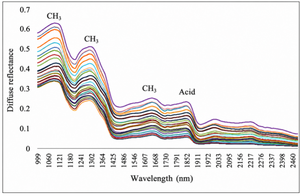
The resulting spectra illustrate the differences in chemical characteristics of each sample type, which are related to variations in the levels of organic matter and dissolved solids in them. Figure 1 displays the spectral features of NIR scans of POME, river water, and irrigation water samples. In general, the POME spectrum shows a higher absorption intensity than river water and irrigation water, reflecting a greater concentration of organic compounds and pollutant load. Conversely, river water and irrigation water show a relatively lower and smoother absorption pattern, indicating a lighter level of pollution. These variations in absorption patterns are an important basis for the process of extracting spectral features and developing prediction models for COD, BOD, and TSS levels using machine learning algorithms.

The spectral image shows several main peaks related to the molecular characteristics of POME, river and irrigation water samples. It should be noted that in aqueous systems, NIR spectra are dominated by water overtone and combination bands (particularly around 1450 nm and 1950 nm), which makes unambiguous assignment of spectral features to specific organic compounds difficult without complementary analytical evidence. The following tentative assignments are therefore offered with caution. The peaks with ranges of 1091–1126, 1270–1320, and 1640–1685 nm may suggest the presence of stretching vibrations and overtones of methyl groups (CH₃) originating from organic compounds such as lipids, fatty acids, and other hydrocarbon compounds commonly found in POME wastewater [31]. The absorption intensity in these regions is higher in POME than in river water and irrigation water, indicating a higher organic matter content.

1.png

Figure 1. Spectral features of palm oil mill effluent (POME), river water and irrigation water

Meanwhile, the peak with a range of 1836–1870 nm may be tentatively related to the combination of O–H and C=O vibrations of carboxylic acids (acid groups), which may suggest the presence of polar compounds, such as organic acids and free fatty acids. These assignments should be interpreted cautiously, as spectral changes in aqueous NIR spectra are frequently influenced by variations in water structure and light scattering rather than direct absorption by specific compounds [32, 33]. This band can also be influenced by the contribution of water molecules, considering that the area is close to the H₂O absorption band. Overall, the presence of these peaks illustrates the differences in chemical composition between sample types and is an important spectral feature that contributes to the development of prediction models for COD, BOD, and TSS levels based on NIR and machine learning.

3.2 Calibration model of chemical oxygen demand contents

Table 2 presents the calibration and validation performance of the developed machine learning models for predicting COD concentrations from NIR spectral data under different spectral preprocessing techniques. The models evaluated include XGB, Ridge regression, Lasso regression, and SVR, each combined with raw spectra as well as MSC, SNV, and SG preprocessing. Model performance is assessed using R², RMSEC, RMSEP, and RPD, providing a comprehensive comparison of model accuracy and robustness across different preprocessing strategies.

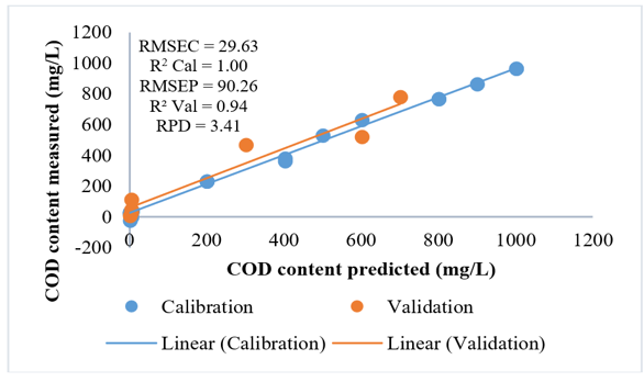
The performance of machine learning models for predicting COD concentrations using NIR spectral data is presented in Table 2. Overall, the results demonstrate that the combination of appropriate preprocessing techniques and machine learning algorithms significantly influences model accuracy. Among all evaluated models, SVR combined with SG preprocessing exhibited the best performance, achieving a validation R² of 0.94 and the lowest RMSEP of 90.26. Additionally, this model produced the highest RPD value of 3.41, indicating excellent predictive capability (see Figure 2). In contrast, SVR models using raw spectra showed poor generalization performance (R² = 0.54), highlighting the importance of spectral preprocessing. This finding confirms that noise reduction and signal enhancement techniques such as SG filtering play a crucial role in improving model robustness. These results are consistent with previous studies reporting that SG preprocessing enhances spectral signal quality and improves prediction accuracy in spectroscopic models [34].

Table 2. Calibration and validation statistics for the prediction of chemical oxygen demand (COD)

2.png

The distribution of COD values (1–1000 mg/L) in this dataset reflects the substantial difference in organic load between raw POME and environmental water samples. This distributional characteristic has important implications for model performance, as the relatively few high-COD POME samples may exert disproportionate influence on the calibration, potentially leading to higher prediction errors at the extremes of the concentration range. The dominance of low-COD samples in the dataset may also bias the model toward better performance in the lower concentration range, which should be considered when interpreting the overall RMSEP values.

A comparison of different machine learning algorithms reveals distinct performance patterns. The XGB model achieved perfect calibration performance (R² = 1.00) across all preprocessing methods; however, its validation performance varied significantly. For instance, XGB with MSC preprocessing achieved R² = 0.88 and RMSEP = 134.99, indicating moderate predictive performance. This discrepancy between calibration and validation results suggests potential overfitting, a common issue in powerful ensemble models such as XGB when applied to relatively small datasets [35]. Similarly, RF-type ensemble behavior (observed in XGB trends) has been reported to produce high training accuracy but may require careful tuning to generalize well. Linear models such as Ridge and Lasso regression showed relatively lower performance compared to nonlinear models. Although Ridge-SG achieved R² = 0.93, its performance was generally less stable across preprocessing methods. This is expected because linear models have limited capability in capturing complex nonlinear relationships between NIR spectra and water quality parameters. Previous studies have also reported that linear regression approaches often underperform compared to nonlinear machine learning models in spectroscopic applications [6].

Spectral preprocessing has a fundamental role in enhancing the performance of predictive models derived from NIR data. Among various preprocessing techniques, SG filtering is widely reported to provide superior performance, particularly when combined with regression-based models such as SVR and Ridge. This advantage is mainly due to its capability to smooth spectral signals by reducing high-frequency noise while preserving important spectral features associated with chemical constituents. Consequently, SG filtering enables better extraction of relevant information from NIR spectra, leading to improved prediction accuracy for water quality parameters such as COD and TSS [36]. Furthermore, SG filtering operates as a polynomial-based smoothing method that minimizes noise without significantly distorting the original signal structure, thereby maintaining meaningful absorption characteristics. This is particularly important in spectroscopic analysis, where subtle variations in spectral features are directly linked to chemical composition [37]. In contrast, raw spectral data are typically affected by various sources of interference, including noise, baseline drift, and scattering effects, which can obscure relevant chemical information and negatively impact model performance. Preprocessing techniques such as SG filtering help mitigate these issues by removing unwanted variations and enhancing signal quality, ultimately leading to more robust and reliable predictive models [38]. Although MSC and SNV preprocessing also contributed to performance improvement by correcting scatter-related variations, their effectiveness was relatively limited compared to SG filtering in this study [39]. This suggests that, for heterogeneous water samples such as POME and environmental water matrices, noise reduction plays a more dominant role than scatter correction in improving model accuracy. These findings highlight the importance of selecting preprocessing strategies that are aligned with both the characteristics of the dataset and the nature of the target parameters, particularly when dealing with complex environmental samples [34].

An important consideration in interpreting the model performance is the potential influence of sample type differences on prediction accuracy. The dataset comprises three distinct sample types—raw POME, river water, and irrigation water—which differ substantially in their physicochemical characteristics and concentration ranges. Consequently, there is a risk that the models may partially learn to discriminate between sample classes rather than capturing the true quantitative relationship between spectral features and COD concentration. This phenomenon, known as class-based confounding, can artificially inflate validation performance metrics when the test set contains samples from all three classes. Nevertheless, the wide COD range covered by the dataset (1–1000 mg/L) and the heterogeneous nature of the samples suggest that the model has been exposed to sufficient spectral variability to learn genuine concentration-related patterns rather than class membership alone.

The use of hold-out validation provided a more realistic assessment of model performance by evaluating the models on the hold-out validation set, thereby reducing the risk of overfitting [40]. The satisfactory validation results indicate that the developed models are capable of maintaining predictive reliability despite the relatively limited dataset size (n = 45), which is a common constraint in environmental monitoring studies. A key strength of this study lies in the inclusion of heterogeneous water samples, such as raw POME, river water, and irrigation water, covering a wide range of contamination levels [3]. This diversity enhances the representativeness of the dataset while also introducing additional complexity due to variations in spectral characteristics across sample types. Despite this challenge, the strong performance of the SVR-SG model demonstrates that machine learning approaches can effectively capture complex and nonlinear relationships within heterogeneous datasets. This highlights the importance of incorporating diverse sample conditions during model development to improve generalizability and ensure practical applicability in real-world environmental monitoring scenarios.

The results of this study demonstrate that the integration of NIR spectroscopy with machine learning provides a rapid and non-destructive approach for COD prediction in POME-contaminated water. The strong predictive performance indicates that the models are capable of capturing spectral features associated with organic compounds contributing to oxygen demand, which are primarily reflected through overtone and combination bands of C–H and O–H bonds in the NIR region [6]. Compared to conventional laboratory methods, which are time-consuming and require chemical reagents, the proposed approach offers significant advantages in terms of analysis speed, cost-efficiency, and environmental sustainability. These benefits are particularly relevant for applications requiring frequent or continuous monitoring. Therefore, the developed method shows strong potential for real-time and in-situ monitoring of organic pollution in POME systems. This capability can support more efficient environmental management and early detection of contamination events in complex water systems [8].

3.3 Calibration model of biochemical oxygen demand contents

Table 3 summarizes the calibration and validation results of machine learning models used to predict BOD concentrations from NIR spectral data, incorporating different preprocessing approaches. The models assessed comprise XGB, Ridge regression, Lasso regression, and SVR, applied to both raw spectra and preprocessed data using MSC, SNV, and SG preprocessing methods. Model performance is assessed using the R², RMSEC, RMSEP, and RPD, allowing for a comprehensive evaluation of predictive accuracy and model robustness across different preprocessing strategies.

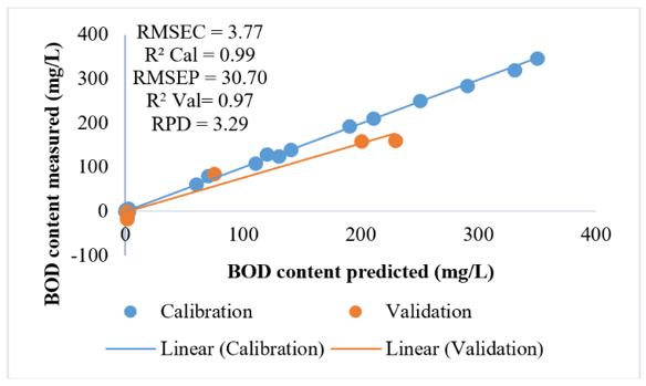
The performance of the developed machine learning models for predicting BOD concentrations is presented in Table 3. Overall, the results indicate that both the choice of algorithm and spectral preprocessing method significantly influence model accuracy and generalization capability. Among all evaluated models, XGB combined with MSC preprocessing exhibited the best predictive performance, achieving a validation R² of 0.97, RMSEP of 30.70, and RPD of 3.29. This result indicates excellent predictive ability, as RPD values greater than 3 are generally considered indicative of robust and reliable models for quantitative prediction (see Figure 3).

Table 3. Calibration and validation statistics for the prediction of biochemical oxygen demand (BOD)

3.png

In contrast, XGB models using raw spectra showed extremely poor validation performance (R² = 0.02), despite achieving perfect calibration accuracy (R² = 1.00). This discrepancy strongly suggests overfitting, where the model captures noise rather than meaningful patterns in the data. Such behavior is commonly observed in powerful ensemble learning algorithms when preprocessing is insufficient or when the dataset is relatively small [35]. The validation R² of XGB-Raw for BOD prediction (R² = 0.02) can be explained by the sensitivity of the XGB algorithm to unprocessed spectral data. Without preprocessing, raw NIR spectra contain substantial baseline drift, multiplicative scattering effects, and inter-sample path length variations that are unrelated to BOD concentration. XGB's decision tree architecture interprets these noise-driven spectral differences as arbitrary splits during training, leading the boosting mechanism to amplify irrelevant patterns. The resulting model memorizes noise-specific features of the training set and fails to generalize to the test set. MSC effectively normalizes these baseline and scattering effects, allowing XGB to focus on genuine BOD-correlated spectral patterns, which explains the dramatic improvement from R² = 0.02 (Raw) to R² = 0.97 (MSC).

The highly skewed distribution of BOD values (0.38–350 mg/L), with the majority of samples clustered at low concentrations and a small number of high-BOD POME samples at the upper tail, introduces additional modeling complexity. High-BOD samples contribute disproportionately to the overall RMSEP, and their limited representation in the dataset may reduce model reliability at extreme concentrations. This distributional imbalance reinforces the importance of collecting additional samples across the full BOD range in future studies to improve calibration robustness.

A comparison across models shows that nonlinear models outperform linear models in predicting BOD from NIR spectra [41, 42]. While Ridge and Lasso regression achieved moderate performance, their validation R² values remained relatively low and inconsistent across preprocessing methods. For example, Ridge regression achieved its best performance with SG preprocessing (R² = 0.87), while Lasso achieved R² = 0.91 with SG. However, both models exhibited unstable performance across different preprocessing methods, indicating limited robustness. On the other hand, nonlinear models such as XGB and SVR demonstrated better adaptability to complex spectral patterns. This finding is consistent with previous studies, which reported that nonlinear machine learning algorithms are more effective in modeling the complex relationships between spectral data and water quality parameters [6].

Spectral preprocessing played a critical role in determining model performance, with MSC providing the most substantial improvement, particularly for the XGB model. This behavior can be attributed to the ability of MSC to effectively correct multiplicative and additive scattering effects caused by variations in particle size, turbidity, and optical path length, which are prominent in heterogeneous water samples containing suspended solids [34]. By normalizing these variations, MSC enhances the consistency of spectral signals, allowing the XGB algorithm to more effectively capture meaningful patterns related to BOD. The superior performance of XGB combined with MSC also reflects the sensitivity of ensemble-based models to input data quality. XGB relies on iterative error minimization through boosting, which can amplify noise and irrelevant variations if the input spectra are not properly corrected. Therefore, the application of MSC helps stabilize the input features, leading to improved model generalization and predictive accuracy. Although SG filtering also improved model performance, particularly for Lasso and SVR models, its impact was slightly less pronounced for XGB in this case. This suggests that, for BOD prediction in heterogeneous water systems, correcting scattering effects is more critical than smoothing high-frequency noise. These findings highlight that the effectiveness of preprocessing techniques is strongly dependent on both the nature of the target parameter and the characteristics of the machine learning algorithm. Similar observations have been reported in previous studies emphasizing the importance of selecting preprocessing strategies tailored to both data properties and modeling approaches [35].

The application of hold-out validation ensures that the reported model performance is reliable and not dependent on a specific data split. The high validation performance of the XGB-MSC model (R² = 0.97) indicates strong generalization capability, even with a relatively small dataset. However, the large variation in performance across preprocessing methods, particularly for XGB, highlights the sensitivity of machine learning models to input data quality. This reinforces the importance of proper preprocessing and model validation in spectroscopic applications.

The relatively wide range of BOD values (0.38–350 mg/L) reflects substantial variability in organic contamination levels across different sample types, including raw POME, river water, and irrigation water. Such variability increases the complexity of the modeling task due to the nonlinear and heterogeneous nature of the underlying chemical and physical processes. However, it also enhances the practical relevance of the developed models by better representing real environmental conditions. The strong performance of the XGB-MSC model suggests that ensemble-based machine learning approaches are capable of effectively capturing complex patterns within heterogeneous datasets [3, 35]. The boosting mechanism in XGB enables the model to iteratively learn from residual errors generated in previous stages, thereby progressively improving predictive performance and adapting to complex data distributions. This sequential learning strategy allows XGB to effectively model nonlinear relationships and interactions among variables, which is particularly beneficial for predicting BOD, a parameter influenced by both biochemical and physicochemical processes [41]. Moreover, the ability of XGB to handle heterogeneous datasets makes it well-suited for environmental applications, where data often originate from diverse sources and exhibit high variability. Studies have shown that incorporating a wide range of environmental conditions during model training enhances the robustness and generalization capability of machine learning models. For instance, ensemble models such as XGB demonstrate strong performance across varying water quality parameters, indicating their capacity to capture complex environmental patterns [43]. Overall, these findings support the notion that both the boosting mechanism of XGB and the use of diverse training datasets are key factors contributing to improved model generalization and predictive accuracy in environmental monitoring applications [44].

Similar to COD prediction, the possibility of class-based confounding should be considered when interpreting BOD prediction results. The three sample types in this study exhibit markedly different BOD ranges—POME samples typically show much higher BOD values compared to river and irrigation water—which means the model may have learned class-specific spectral signatures in addition to genuine BOD-related features. The strong performance of XGB-MSC (R² = 0.97) may therefore partly reflect the model's ability to distinguish POME from environmental water samples based on overall spectral intensity differences, rather than purely from BOD-correlated absorption features. Future studies should include a leave-one-type-out validation to rigorously evaluate the model's ability to predict BOD across previously the hold-out validation set sample types.

The results demonstrate that the integration of NIR spectroscopy with machine learning, particularly XGB combined with MSC preprocessing, provides a reliable and efficient approach for predicting BOD in POME-contaminated water. The high predictive performance achieved by the model indicates its capability to capture complex relationships between spectral features and biodegradable organic content [6, 35]. Compared to conventional BOD analysis, which requires a standard incubation period of five days, the proposed method offers a significantly faster alternative while maintaining a high level of accuracy. This substantial reduction in analysis time highlights the potential of the approach for near real-time monitoring applications. Such capability is particularly valuable in palm oil-producing regions, where continuous monitoring of effluent discharge is essential to prevent environmental degradation. Therefore, the proposed method can support more efficient decision-making and pollution management strategies. These findings are consistent with previous studies highlighting the advantages of spectroscopy-based techniques for rapid water quality assessment [7].

3.4 Calibration model of total suspended solids content

The predictive capability of the developed models was evaluated using NIR spectral data under different preprocessing strategies. Table 4 reports the calibration and validation performance of the machine learning models for estimating TSS concentrations. Overall, the results indicate that model performance is strongly influenced by the choice of preprocessing technique, with certain methods yielding improved accuracy and robustness in both calibration and validation stages. The evaluated models include XGB, Ridge regression, Lasso regression, and SVR, combined with raw spectra as well as MSC, SNV, and SG preprocessing methods. Model performance is assessed using R², RMSEC, RMSEP, and RPD, providing a comprehensive comparison of model accuracy and robustness across different preprocessing strategies.

The performance of machine learning models for predicting TSS concentrations based on NIR spectral data is presented in Table 4. The results show that model performance varies considerably depending on both the selected algorithm and the applied spectral preprocessing method. Among all evaluated models, SVR combined with SG preprocessing achieved the best overall performance, with a validation R² of 0.85, RMSEP of 52.10, and RPD of 2.39. This indicates a good predictive capability, as RPD values between 2.0 and 3.0 are generally considered suitable for quantitative prediction in environmental applications (see Figure 4). In contrast, SVR models using MSC preprocessing showed very poor performance (R² = 0.03), highlighting the strong dependency of model performance on preprocessing strategy. This result emphasizes the importance of selecting appropriate preprocessing techniques to extract meaningful information from spectral data. The poor performance of SVR-MSC for TSS prediction (R² = 0.03) can be attributed to the fundamental mismatch between the MSC correction mechanism and the physical nature of TSS. TSS is primarily governed by light scattering from suspended particles, meaning that scattering-related spectral variations carry direct analytical information about suspended solid concentration. MSC was designed to remove multiplicative scattering effects by normalizing spectra against a reference. However, this normalization inadvertently removes the scattering information that correlates with TSS. This effectively destroys the signal of interest, leaving the SVR model with insufficient spectral information to build a meaningful calibration. In contrast, SG first-derivative transformation preserves scattering-related spectral differences while removing baseline offsets, which explains the superior performance of SVR-SG for TSS prediction.

Table 4. Calibration and validation statistics for the prediction of total suspended solids (TSS)

4.png

The TSS distribution (8.7–709 mg/L) is similarly right-skewed, driven by the high suspended solid content of raw POME samples. The uneven distribution of samples across the concentration range may affect model generalizability, particularly at high TSS values where the relationship between light scattering and spectral response becomes increasingly nonlinear. Future studies should aim for a more balanced representation of samples across the full TSS range to improve model robustness.

A comparison across different algorithms reveals that nonlinear models again outperform linear models, although the performance gap is less pronounced than in COD and BOD prediction. The XGB model showed strong calibration performance (R² ≈ 1.00), but its validation results were inconsistent. For example, XGB-SG achieved R² = 0.86, while XGB-MSC dropped significantly to R² = 0.21. This pattern suggests that XGB is highly sensitive to preprocessing and may suffer from overfitting when the input data are not optimally conditioned. Linear models such as Ridge and Lasso regression exhibited relatively lower and more stable performance, with validation R² values generally ranging between 0.39 and 0.81. However, their inability to capture nonlinear relationships limits their predictive accuracy compared to nonlinear approaches. These findings are consistent with previous studies indicating that nonlinear machine learning models are better suited for handling complex spectral data and heterogeneous environmental samples [6].

Spectral preprocessing plays a crucial role in improving model performance for TSS prediction, which is predominantly governed by physical rather than chemical characteristics of the samples. Among the evaluated preprocessing techniques, SG filtering consistently enhanced model performance, particularly for SVR and XGB models. This improvement can be attributed to the ability of SG filtering to effectively reduce high-frequency noise while preserving important spectral features related to light scattering caused by suspended particles. Such preservation is essential because these scattering-induced variations carry significant information about the physical properties of the sample [21]. In contrast, MSC and SNV preprocessing showed inconsistent effects across models. In some cases, such as SVR-MSC, preprocessing resulted in a significant decline in performance, suggesting that excessive correction of scattering effects may inadvertently remove relevant information linked to suspended solids. This highlights the importance of selecting preprocessing techniques that are aligned with the underlying nature of the target parameter. For TSS prediction, where scattering effects carry meaningful information, noise smoothing appears to be more beneficial than aggressive scatter correction. These findings are consistent with previous studies emphasizing the critical role of appropriate preprocessing strategies in spectroscopic modeling [34].

The use of hold-out validation provides a more reliable assessment of model robustness than calibration statistics alone, because performance is evaluated on samples excluded from model fitting. The satisfactory validation performance achieved by the SVR-SG model indicates its ability to generalize beyond the calibration dataset, despite the relatively limited sample size. This suggests that the model is capable of capturing the underlying relationships between spectral features and target variables rather than merely fitting noise [44, 45]. However, the variability in model performance observed across different preprocessing techniques highlights the sensitivity of spectroscopic machine learning models to data quality and feature conditioning. Spectral preprocessing plays a critical role in shaping the input feature space, and inappropriate preprocessing can either suppress relevant information or retain unwanted noise and artifacts, ultimately affecting model accuracy and stability. This sensitivity reflects the strong dependence of model performance on how well the preprocessing techniques preserve relevant spectral information while minimizing noise and distortions. Therefore, careful selection and optimization of preprocessing strategies are essential to ensure robust and reliable predictions in spectroscopic applications, particularly when dealing with heterogeneous environmental datasets [6, 34].

The potential for class-based confounding is particularly relevant for TSS prediction, given that TSS is predominantly governed by physical scattering characteristics rather than specific chemical absorption features. POME samples typically contain significantly higher suspended solid loads compared to river and irrigation water, creating distinct spectral signatures associated with turbidity and particle scattering. While the SVR-SG model achieved satisfactory validation performance, it cannot be excluded that part of this performance reflects discrimination between high-turbidity POME and lower-turbidity environmental water samples. A per-class RMSEP analysis and leave-one-type-out validation would provide more definitive evidence of the model's ability to generalize across different water matrices, and is recommended as a priority for future work.

The TSS concentration range (8.7–709 mg/L) reflects substantial variability in suspended solids across different sample types, including raw POME, river water, and irrigation water. This variability introduces significant modeling challenges due to differences in particle size distribution, turbidity, and optical properties, all of which influence light scattering behavior in the NIR region. Despite these complexities, the relatively strong performance of the SVR-SG model suggests that machine learning approaches are capable of capturing the indirect and nonlinear relationships between scattering-related spectral features and TSS levels. The ability of SVR to model complex feature spaces, combined with the noise-reducing capability of SG filtering, likely contributed to this performance. The inclusion of heterogeneous samples further enhances the robustness of the developed models by exposing them to a broader range of environmental conditions during training. This improves their generalizability and practical applicability in real-world monitoring scenarios. These findings support previous studies emphasizing that incorporating diverse datasets is essential for developing reliable spectroscopic models in environmental applications.

The results confirm that the integration of NIR spectroscopy with machine learning provides a feasible and efficient approach for the rapid prediction of TSS in POME-contaminated water systems. The ability of the model to capture scattering-related spectral features associated with suspended particles highlights its effectiveness in estimating TSS, which is primarily governed by physical properties rather than chemical composition. Compared to conventional gravimetric methods, which are labor-intensive and require extensive laboratory procedures, the proposed approach offers a significantly faster and more efficient alternative while maintaining satisfactory predictive performance. This advantage is particularly important for applications requiring near real-time monitoring, where timely information is critical for environmental management and pollution control. Therefore, the developed method has strong potential to support continuous monitoring systems in complex environmental settings. These findings are consistent with previous studies highlighting the benefits of spectroscopic techniques for rapid water quality assessment [7].