
Imad Habeeb Obead | Marwah Jaafar Kashkool*
© 2026 The authors. This article is published by IIETA and is licensed under the CC BY 4.0 license (http://creativecommons.org/licenses/by/4.0/).
OPEN ACCESS
This study develops a coupled simulation-optimization methodology for seasonal water-quality management of a 42.5 km reach of the Kufa River, Iraq, where six point discharges interact with three drinking-water intakes under wet- and dry-season flow. A calibrated MIKE 11 model was reduced to seasonal linear response matrices linking removal ratios at three controllable sources to concentrations at all evaluation stations, and the allocation was solved as a five-objective problem with NSGA-II. The Iraqi Standard Specification IQS 417/2009 limits for Total Dissolved Solids (TDS), Biochemical Oxygen Demand (BOD), and NO3 are imposed as hard constraints at the two intakes that lie downstream of the controllable sources, whereas phosphate is carried as a penalty objective rather than a hard constraint because its 0.5 mg/L guideline cannot be met at the intakes in the dry season within feasible treatment intensities, and enforcing it would leave no admissible solution. All 77 Pareto-optimal solutions satisfied the TDS, BOD, and NO3 limits at both intakes in both seasons with zero exceedance. Phosphate is the dominant pressure: dry-season residues of 0.20 to 0.43 mg/L remain above the guideline at the intakes under every solution, while wet-season dilution removes them. A compromise solution, selected by minimum normalized distance to the ideal point over all five objectives and unchanged under alternative criteria, secures most of the achievable risk reduction for about a quarter of the achievable increase in removal effort and is put forward as a preliminary reference scenario. The results suggest that the TDS, BOD and NO3 intake limits may be attainable with removal ratios not exceeding 0.80, subject to validation of the response matrices against the full model, and the framework offers a transferable template for seasonal load allocation in multi-intake river systems.
Kufa River, MIKE 11, NSGA-II, response-matrix model, seasonal water-quality management, waste-load allocation
The rivers of the lower Euphrates basin serve as the main source of municipal drinking water, irrigation water, and the actual outfall of urban and agricultural runoff. This role creates essential tension: the same section that must deliver drinking water at the intake points also accommodates untreated or partially treated point discharges whose loads are largely insensitive to river flow, such that ambient concentrations increase as river discharge decreases. In Iraq, where upstream regulation, frequent droughts, and climate change have reduced Euphrates inflows and increased annual variability, this stress has accelerated from a concern to a critical operational problem [1, 2].
The traditional response to this problem is pollutant load distribution: determining how much each point source must reduce its pollutant load so that standards are met at specific control points, at the lowest cost or according to some principle of equity [3, 4]. Early formulations relied on linear or dynamic programming coupled with Streeter-Phelps analytical water-quality relations. Present practice has shifted to simulation planning examples in which a process-based hydrodynamic and water quality model capable of representing rebound, lateral withdrawal, seasonal limit conditions, and multi-component transition effects is coupled with a community-based metaheuristic algorithm that does not require derivative information [5-7]. Multi-objective evolutionary algorithms, particularly NSGA-II, have become the major standard because water quality management is inherently multi-objective [8]: regulatory compliance, treatment costs, service levels at intakes, and the spatial distribution of residual pollution are partially conflicting objectives that cannot be a priori combined into a single metric function. However, a recurring methodological weakness in the applied literature concerns the handling of regulatory boundaries. In many studies, the criteria are included as penalty limits within the objective functions, that is, as flexible constraints allowing the optimizer to trade off minor violations for cost savings. While the flexible assumption is computationally convenient, it is unsuitable where the control points are drinking water intakes, since drinking water limits are legally binding, and a “slightly non-compliant” distribution has no operational significance. On the other hand, imposing a strict limit at every station could deplete the usable area when certain components, typically feeders under low-flow conditions, are physically uncontrollable under realistic treatment intensities. Therefore, a practical approach is needed: strict limits are required where legal compliance is needed (at the intakes), and a penalty-based approach for components whose limits may be unmanageable under drought hydrology. This research develops precisely such a formulation for the Kufa River, a tributary of the Euphrates that feeds the Kufa catchment, and presents a complete analysis of the strict limitation situation at the intakes. The contributions are: (1) Reducing the calibrated and verified MIKE 11 hydrodynamic model DHI [9] for the section to a seasonal linear response-matrix model that predicts multi-component concentrations at all assessment stations as an explicit function of removal ratios at controllable sources, thereby reducing the cost of each target assessment by several orders of magnitude while preserving the physics embedded in the complete model. (2) Formulating the management issue as a five-objective program: environmental risk, treatment cost, intake water quality index, spatial equity, and allocated squared phosphate penalty, with IQS 417/2009 [10] limits on Total Dissolved Solids (TDS), Biochemical Oxygen Demand (BOD), and NO3 imposing strict nonlinear constraints at the intakes in both seasons. (3) The problem was solved by the NSGA-II algorithm, and the resulting Pareto set was divided into five representative solutions, each examined component by component, intake by intake, and season by season. (4) Phosphate was isolated as the governing component of the system, and its seasonal irregularity in finite controllability was determined, yielding a direct practical guide to the investment phase of the treatment. Based on our literature review, the combination of strict intake-level constraints, a season-specific response matrix, and a five-objective evolutionary search has not previously been reported for the Kufa River or for comparable Euphrates distributaries. The individual components are established; the contribution of this work lies in their integration under an explicit seasonal, multi-intake, mixed constraint formulation.
2.1 Kufa River section
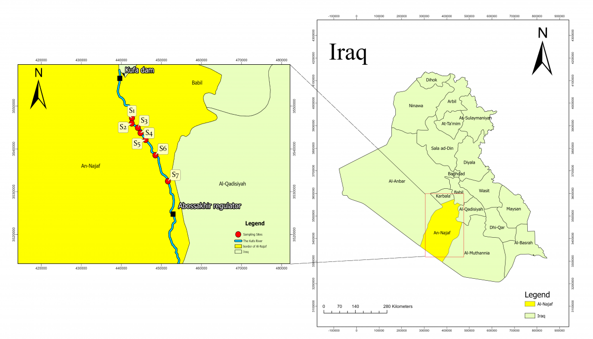
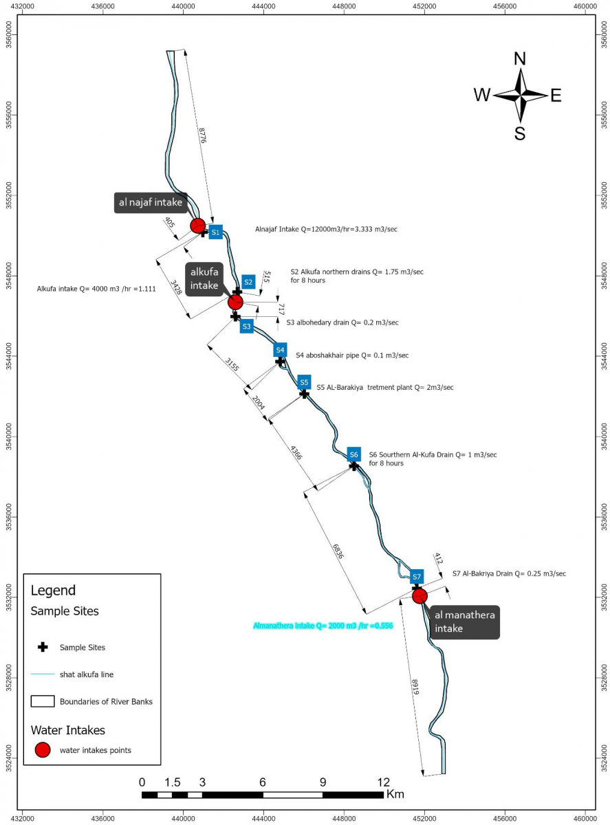
The Euphrates River branches into the Kufa and Abbasia branches in the upper reaches of Najaf Governorate. The Kufa River flows for a distance of 75.2 km within the governorate through the districts of Kufa, Manadhira, and Mishkhab, providing drinking, industrial, and irrigation water Kareem and Alkatib [11]. The population of Al-Najaf governorate exceeds 1.9 million according to the 2024 census data issued by the Iraqi Ministry of Planning's Statistics Authority (2024). The study section extends 42.467 km from the Kufa barrage (station 0 + 00) to the Abu Sukhair regulator, including three main intakes: Najaf intake at Zarqa region with a discharge of 3.333 m3/sec (withdrawal), Kufa intake (1.111 m3/sec- withdrawal), and Manadhira intake (0.556 m3/sec- withdrawal) with seven-point discharge sources (S1-S7) involving drains, municipal water, pipes, and pumping stations. The largest discharge is the Barakiya outfall S5 (1.157 m3/sec), followed by the northern Kufa drain S2 (0.583 m3/sec). The irregular intake and discharge mean that concentrations at each intake are not governed by a single source, but rather by the cumulative mass balance of mixing, longitudinal diffusion, biochemical transformation, and runoff, making management a hydrodynamic and water quality-related distribution issue. Figure 1 shows the study area within the Al-Najaf governorate in Iraq, and Figure 2 shows the location of the stations along the Kufa River reach, after [12]. Table 1 shows the longitudinal orders of the sources and intakes along the study reach.
Figure 1. Layout map of Iraq and the Al-Najaf governorate
Figure 2. Layout map for the study stations along the Kufa River reach
Table 1. Longitudinal positions of the point sources and intakes along the study reach
|
Code |
Description |
Branch |
Station (km) |
Function and Discharge (m3/sec) |
|
- |
Kufa Barrage |
Kufa |
0 + 00 |
Upstream boundary |
|
S1 |
Al-Zarqa water intake (Najaf intake) |
Kufa |
9 + 662 |
Withdrawal, 3.333; not constrained |
|
S2 |
Northern Al-Kufa drain |
Kufa |
13 + 846 |
Point discharge, 0.583 |
|
- |
Kufa water intake |
Kufa |
14 + 372 |
Withdrawal, 1.111; strict constraint |
|
S3 |
Albo-Hedary drain |
Kufa |
14 + 976 |
Controllable discharge, 0.200 |
|
S4 |
Alboshakhair pipe |
Alboshakhair |
18 + 324 |
Controllable discharge, 0.100 |
|
S5 |
Al-Barakiya treatment plant |
Kufa |
20 + 403 |
Controllable discharge, 1.157 |
|
S6 |
Southern Al-Kufa drain |
Albo-Issa |
25 + 171 |
Point discharge, 0.333 |
|
S7 |
Al-Bakriya drain |
Kufa |
32 + 363 |
Point discharge, 0.250 |
|
- |
Al-Manadhira water intake |
Kufa |
32 + 735 |
Withdrawal, 0.556; strict constraint |
|
- |
Abu Sukhair regulator |
Kufa |
42 + 468 |
Downstream boundary |
Note: “–” denotes boundary or intake locations without a source-station code.
2.2 Flow systems
Table 2 presents the multiple flow systems identified statistically from extreme flow frequency analysis of annual flow records for the period 2004-2022, which is the period over which the reach was characterized for the present management analysis.
Table 2. Descriptive statistics for annual flow records (2004–2022) for the Kufa River
|
Discharge |
Minimum (m3/sec) |
Maximum (m3/sec) |
Mean (m3/sec) |
Standard Deviation (m3/sec) |
|
Annual Maximum |
100.667 |
255.161 |
155.091 |
43.636 |
|
Annual Minimum |
34.032 |
99.548 |
62.313 |
20.147 |
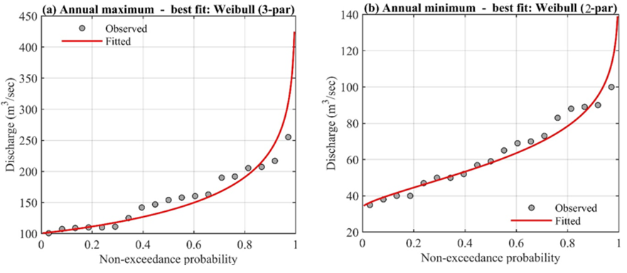
From the results of Table 2, it is evident that the large standard deviations reflect the high annual variability and the river flow sensitivity to climatic stress. Frequency analysis with the two-parameter Weibull distribution for the annual maximum series and the three-parameter Weibull distribution for the annual minimum series provided design discharges to simulate extreme conditions: a 50-year minimum discharge of 30.495 m3/sec (for the dry scenario) and a 50-year maximum discharge of 243.159 m3/sec (for the flood scenario), surrounding the normal operation of the calibrated baseline. These 50-year quantiles are extrapolated from a 19-year record and are therefore used only as specific hydraulic stress scenarios; the water-quality optimization described below is performed on the calibrated seasonal baseline states corresponding to the two sampling rounds, not on the 50-year quantiles.
The frequency analysis for two design discharges is given in Table 3.
Seven probability distributions were fitted to each series by maximum likelihood and ranked by the Akaike information criterion, with the Bayesian criterion, the Kolmogorov-Smirnov and Anderson-Darling probabilities and confidence intervals presented in Table 3. Every distribution is accepted by the Kolmogorov–Smirnov test at the 5% level; the whole ΔAIC range is 5.29 for the maximum series and only 2.24 for the minimum series. For n = 19, such differences are not evidence of a preferred model. More importantly for the use made of these quantiles here, the design discharges adopted in this work, 243.159 and 30.495 m3/sec, lie inside the ninety-five per cent confidence interval of all seven candidates in both series, so the choice of distribution does not materially alter the flow scenarios or any result that follows from them.
Table 3. Comparison of probability distributions fitted to the annual maximum and annual minimum series of the Kufa River, 2004–2022
|
Distribution |
k |
AIC |
ΔAIC |
KS |
AD |
95 % CI (m3/sec) |
|
(a) Annual maximum series (n = 19) |
||||||
|
Weibull (3) |
3 |
196.40 |
0.00 |
0.576 |
0.046 |
230.0-633.1 |
|
Gumbel |
2 |
199.34 |
2.94 |
0.511 |
0.125 |
215.2-322.7 |
|
Log-normal |
2 |
199.43 |
3.03 |
0.587 |
0.209 |
215.2-317.5 |
|
Gamma |
2 |
199.78 |
3.38 |
0.569 |
0.174 |
209.4-296.9 |
|
Log-Pearson III |
3 |
201.27 |
4.87 |
0.578 |
0.199 |
223.4-316.5 |
|
GEV |
3 |
201.29 |
4.89 |
0.506 |
0.111 |
206.8-unbounded |
|
Weibull (2) |
2 |
201.69 |
5.29 |
0.777 |
0.172 |
204.9-277.3 |
|
(b) Annual minimum series (n = 19) |
||||||
|
Weibull (3) |
3 |
169.51 |
0.00 |
0.962 |
0.458 |
24.7- 40.8 |
|
Gamma |
2 |
169.66 |
0.15 |
0.957 |
0.473 |
24.1-38.3 |
|
Log-normal |
2 |
169.69 |
0.18 |
0.977 |
0.560 |
26.0-39.0 |
|
Gumbel |
2 |
169.91 |
0.40 |
0.958 |
0.471 |
26.5-40.0 |
|
Weibull (2) |
2 |
170.42 |
0.91 |
0.896 |
0.363 |
17.4-33.7 |
|
Log-Pearson III |
3 |
171.67 |
2.16 |
0.000 |
1.000 |
26.7-37.9 |
|
GEV |
3 |
171.75 |
2.24 |
0.939 |
0.416 |
-35.0-38.5 |
Note: k is the number of fitted parameters. ΔAIC is measured from the lowest value within each class. KS and AD are the Kolmogorov-Smirnov and Anderson-Darling probabilities; a value above 0.05 indicates that the fit is not rejected.
The two-parameter Weibull distribution was adopted for the annual maximum series, and the three-parameter Weibull distribution was adopted for the annual minimum series, for consistency with the antecedent hydrological analysis of the same reach [13] and because both yield stable intervals; the two-parameter form gives the narrowest interval of all seven candidates for the maxima, 204.9 to 277.3 m3/sec. Two probability distributions were examined and set aside on grounds of numerical behavior rather than fit. The generalized extreme value distribution returns an effectively unbounded upper confidence limit for the maximum series and a physically impossible negative lower limit for the minimum series, both symptomatic of an unconstrained shape parameter on a short record. The log-Pearson type III fit to the minimum series is rejected by the Kolmogorov–Smirnov test, and its Anderson-Darling probability of unity is an artefact of a negative fitted skew rather than evidence of a good fit.
The three-parameter Weibull attains the lowest AIC in both panels, but by margins of 2.94 and 0.15, respectively, and its location parameter is determined almost entirely by the smallest observation, so the fitted 50-year minimum is sensitive to a single data point. The intervals themselves are wide, covering 29% of the point estimate for the adopted maximum and 45% for the adopted minimum. Probability plots of the best-fitting distribution for the annual maximum and annual minimum series are shown in Figure 3.
Figure 3. Fitted probability distributions for the discharge series, 2004–2022: (a) Annual maximum and (b) annual minimum
Table 4 states the correspondence between flow scenarios, simulation purpose, and water-quality data.
Table 4. Assignment of simulations and water-quality observations to flow scenarios
|
Flow Scenario |
Discharge (m3/sec) |
Simulation Module and Purpose |
Water-Quality Data Set |
|
50-year minimum |
30.495 |
HD only; lower bound of stage, velocity and travel time |
None |
|
Calibrated dry baseline |
130.96 |
HD + AD + ECO Lab; basis of Adry and of the dry-season optimization |
Dry-season round |
|
Calibrated wet baseline |
97.64 |
HD + AD + ECO Lab; basis of Awet and of the wet-season optimization |
Wet-season round |
|
50-year maximum |
243.159 |
HD only; upper bound of stage, velocity and travel time |
None |
Note: HD: hydrodynamic module; AD: Advection–Dispersion module; ECO Lab: Ecological Laboratory module.
2.3 Water quality monitoring and governing standards
Water samples were collected at seven monitoring stations, S1–S7, of which S2–S7 represent point discharges, and S1 represents the Al-Zarqa water intake, during both the wet and dry seasons and analyzed for a series of physicochemical properties. The four components transferred to the management model, TDS, BOD, NO3, and PO4, were adopted because they combine importance (all limited by the Iraqi Quality Standard IQS for drinking water) with strong sensitivity to both point load and river flow. Tables 5 and 6 show the seasonal baseline concentrations at the monitoring stations. Samples were collected from 22 sites in two rounds, in March 2024 for the wet season and in August 2024 for the dry season. For each point discharge, samples were collected at the discharge location and at points 50 m upstream and 50 m downstream, so that the local effect of each source can be separated from the ambient river concentration; an additional station was located 750 m upstream of the Alboshakhair pipe (S4). Site coordinates were fixed by GPS, samples were stored in coded, pre-rinsed 1.5 L bottles and transported to the laboratory, and 22 parameters were determined and compared against the Iraqi and WHO drinking-water standards; four were carried into the management model. A single round was taken in each season; this is a limitation of the field program and is reflected in the deterministic treatment of the source terms throughout. Because an allocation problem is governed by mass rather than by concentration, the load of each discharge, L = 86.4 QC, was computed from the discharges of Table 1: in the wet season S5 carries 56% of the solids load and 83% of the PO4 load, S2 ranks second on solids at 17% and S7 second on PO4 at 8%, while in the dry season the totals fall to 77% and 20% of their wet-season values and the distribution flattens, the share of S5 dropping to 49% and 45% as that of S2 rises to 18% and 20% (Tables 7 and 8).
Table 5. Basic concentrations of modeled components, wet season (mg/L)
|
Stations |
TDS |
BOD |
NO3 |
PO4 |
|
S1 (Zarqa) |
1153.2 |
5.8 |
2.562 |
0.122 |
|
S2 |
1174.6 |
3.8 |
1.256 |
0.334 |
|
S3 (Albo-Hedary drain) |
1452.2 |
3.4 |
3.353 |
2.294 |
|
S4 (Alboshakhair pipe) |
1195.9 |
4.2 |
1.939 |
0.440 |
|
S5 (Al-Barakiya) |
1943.4 |
3.6 |
3.108 |
9.127 |
|
S6 |
1174.6 |
3.4 |
3.008 |
1.393 |
|
S7 (Al-Bakriya drain) |
1089.2 |
1.6 |
2.461 |
4.040 |
Table 6. Basic concentrations of modeled components, dry season (mg/L)
|
Stations |
TDS |
BOD |
NO3 |
PO4 |
|
S1 (Zarqa) |
961 |
0.8 |
2.687 |
0.652 |
|
S2 |
982 |
1.8 |
1.882 |
0.863 |
|
S3 (Albo-Hedary drain) |
1111 |
0.8 |
0.449 |
1.446 |
|
S4 (Alboshakhair pipe) |
1225 |
0.4 |
2.113 |
0.334 |
|
S5 (Al-Barakiya) |
1303 |
1.0 |
1.955 |
0.969 |
|
S6 |
1192 |
1.8 |
1.982 |
0.952 |
|
S7 (Al-Bakriya drain) |
1105 |
0.8 |
2.457 |
0.873 |
Note: TDS: Total Dissolved Solids; BOD: Biochemical Oxygen Demand.
Table 7. Wet-season pollutant loads of the six point discharges (kg/d)
|
Source |
Discharge (m3/sec) |
TDS |
BOD |
NO3 |
PO4 |
% of Wet TDS Load |
% of Wet PO4 Load |
|
S2 |
0.583 |
59166 |
191.4 |
63.3 |
16.8 |
17.1 |
1.5 |
|
S3 |
0.200 |
25094 |
58.8 |
57.9 |
39.6 |
7.2 |
3.6 |
|
S4 |
0.100 |
10333 |
36.3 |
16.8 |
3.8 |
3.0 |
0.3 |
|
S5 |
1.157 |
194272 |
359.9 |
310.7 |
912.4 |
56.1 |
82.9 |
|
S6 |
0.333 |
33795 |
97.8 |
86.5 |
40.1 |
9.8 |
3.6 |
|
S7 |
0.250 |
23527 |
34.6 |
53.2 |
87.3 |
6.8 |
7.9 |
|
Total |
2.623 |
346186 |
778.7 |
588.4 |
1100.0 |
100.0 |
100.0 |
Note: TDS: Total Dissolved Solids; BOD: Biochemical Oxygen Demand.
Table 8. Dry-season pollutant loads of the six point discharges (kg/d)
|
Source |
Discharge (m3/sec) |
TDS |
BOD |
NO3 |
PO4 |
% of Dry TDS Load |
% of Dry PO4 Load |
|
S2 |
0.583 |
49465 |
90.7 |
94.8 |
43.5 |
18.5 |
20.3 |
|
S3 |
0.200 |
19198 |
13.8 |
7.8 |
25.0 |
7.2 |
11.7 |
|
S4 |
0.100 |
10584 |
3.5 |
18.3 |
2.9 |
4.0 |
1.3 |
|
S5 |
1.157 |
130254 |
100.0 |
195.4 |
96.9 |
48.7 |
45.2 |
|
S6 |
0.333 |
34295 |
51.8 |
57.0 |
27.4 |
12.8 |
12.8 |
|
S7 |
0.250 |
23868 |
17.3 |
53.1 |
18.9 |
8.9 |
8.8 |
|
Total |
2.623 |
267664 |
277.0 |
426.3 |
214.5 |
100.0 |
100.0 |
Note: TDS: Total Dissolved Solids; BOD: Biochemical Oxygen Demand.
Table 9. Inspection of the six-point discharges against the selection criteria
|
Source |
Discharge (m3/sec) |
TDS Load Rank |
Decision |
Basis of the Decision* |
|
S2 |
0.583 |
2 |
No |
Municipal drain. |
|
S3 |
0.200 |
4 |
Yes |
Discrete outfall under a single authority. |
|
S4 |
0.100 |
6 |
Yes |
Discrete pipe outfall under a single authority. |
|
S5 |
1.157 |
1 |
Yes |
Existing treatment plant, overloaded; largest load on the reach. |
|
S6 |
0.333 |
3 |
No |
On the Albo-Issa branch. |
|
S7 |
0.250 |
5 |
No |
Second-highest wet-season PO4 concentration. |
Note: *The basis of the selection is administrative rather than hydraulic. TDS: Total Dissolved Solids.
The wet season carries the most severe source loading at S5 (Al-Barakiya): TDS = 1943 mg/L, and PO4 = 9.127 mg/L, values that far exceed drinking water limits and establish S5 as the main pollution stress for the section. High PO4 is also observed at S7 (4.04 mg/L) and S3 (2.294 mg/L). In the dry season, absolute TDS is generally lower, but chemical concentrations remain concerning, and reduced dilution increases the effect of each source, thus contributing to the seasonal irregularity. Averaged over the three controllable sources, the wet-season baselines exceed the dry-season values by factors of 1.26 for TDS, 5.09 for BOD, 1.86 for nitrate, and 4.31 for phosphate. This reversal of the usual dilution expectation is consistent with the wet-season round agreeing with the irrigation-drainage return-flow period, when the drains convey leached salts and fertilizer-derived nitrogen and phosphorus from the surrounding irrigated land.
The standard limits exerted at the intakes are the drinking water values according to the IQS417/2009: TDS ≤ 1000 mg/L, BOD ≤ 6 mg/L, and NO3 ≤ 50 mg/L, applied equally in both seasons. Phosphates are controlled with an objective limit of 0.5 mg/L (consistent with the WHO guideline value; the strictest environmental value in the IQS is 0.4 mg/L), but are treated with a penalty rather than a strict restriction.
2.4 Selection of controllable sources and constrained intakes
Three of the six point discharges, S3, S4 and S5, are treated as controllable. Table 9 shows the position, discharge, and load rank of each source, along with the basis for the decision.
3.1 MIKE 11 hydrodynamic model and water quality
The physical basis of the methodology is the MIKE 11 model of the study section, which combines three modules: the hydrodynamic module (HD), which solves the one-dimensional Saint-Venant equations for water level and discharge along the branching network; the advection–dispersion module (AD), which transports dissolved components; and the Ecological Laboratory module (ECO Lab), which represents biochemical transformations (particularly BOD decay and its associated DO dynamics). River cross-sections, bottom slopes, and the limiting conditions of the barrage, regulator, and lateral intake and discharge structures (presented in Figure 2) were coded from field surveys and official administrative records. The model simulates the complete nonlinear interaction between runoff at intakes, lateral loading at drains, and the longitudinal diffusion and decay that govern intake concentrations.
3.2 Calibration and verification
The HD was calibrated at the water levels observed at the Kufa and Al-Manadhira stations for March 2023, and verified for August 2024. The construction and calibration of this model, including the treatment of extreme flow conditions on the same reach, are reported in full by Kashkool and Obead [13]; the present work adopts the calibrated configuration described there and extends it to the seasonal allocation problem. The Manning roughness coefficient was taken as the main control variable, and the diffusion coefficient in the AD module and the decay coefficient in the ECO Lab were adjusted by trial and error. Performance was evaluated using the coefficient of determination (R2), root mean square error (RMSE), ratio of RMSE to the standard deviation of observations (RSR), and percentage bias (PBIAS), as quoted by Moriasi et al. [14]; the roughness trials are summarized in Table 10 and the performance of the adopted value in Table 11.
The adopted roughness, n = 0.02445, gave the highest coefficient of determination at both stations (Table 10), with R2 of 0.965 at Kufa and 0.920 at Al-Manadhira, and RMSE of 0.655 and 0.354 m, respectively [13]. The diffusion coefficient ranged from 50 to 100 m2/sec, while the first-order decay coefficient was calibrated to 1.0 day-1. The RSR values of 2.772 and 0.976 fall in the unsatisfactory group of the Moriasi [14] classification, yet the R2 values of 0.965 and 0.920 show that the model reproduces the observed pattern closely. The two statements are bounded by the bias: at Kufa the mean balance between simulated and observed stage is +0.653 m against an RMSE of 0.655 m, so the error is almost entirely a constant offset, and the RMSE falls to 0.051 m once it is removed. The offset is consistent with a difference between the datum of the gauge record and that of the model, and it is compounded by the narrow, barrage-controlled range of the observed stage, which reduces the denominator of RSR. Because the response matrix operates on deviations from the calibrated baseline rather than on absolute stage, a constant offset cancels in the allocation results, while the remaining bias is reported through PBIAS in Table 11.
Table 10. Coefficient of determination for the trial values of Manning’s roughness coefficient (based on water level records)
|
Manning’s Coefficients n (sec·m-1/3) |
Statistics |
Kufa Station |
Al-Manadhira Station |
|
0.033 |
R2 |
94% |
90% |
|
0.02 |
R2 |
95% |
91% |
|
0.02445 (adopted) |
R2 |
96% |
92% |
Note: The error statistics of the adopted roughness (RMSE, RSR and PBIAS) are reported in Table 11.
Table 11. Hydrodynamic calibration and validation performance
|
Statistic* |
Kufa Station (Calibration, March 2023) |
Al-Manadhira Station (Validation, August 2024) |
|
Adopted Manning n (sec·m-1/3) |
0.02445 |
0.02445 |
|
Number of daily observations |
31 |
31 |
|
R2 |
0.965 |
0.920 |
|
RMSE (m) |
0.655 |
0.354 |
|
Systematic bias (m) |
+0.653 |
+0.338 |
|
RMSE after removal of the bias (m) |
0.051 |
0.105 |
|
RSR |
2.772 |
0.976 |
|
PBIAS (%) |
-3.30 |
-1.87 |
Note: Root mean square error (RMSE). *Statistics for the adopted roughness are taken from Kashkool and Obead [13]. The bias and the debiased RMSE were computed from the daily observed and simulated water levels. PBIAS = 100 × Σ(Oᵢ − Sᵢ)/ΣOᵢ, where Oᵢ and Sᵢ are the observed and simulated water levels on day i; a negative value indicates that the model overestimates the observed stage [14].
The advection-dispersion module was calibrated on TDS, the conservative, and the ECO Lab module on the reactive, at four stations covering the reach. Calibration used March 2023 and verification August 2024 as given in Table 12.
Table 12. Water-quality calibration statistics at the four monitoring stations, March 2023
|
Station |
Statistic |
TDS |
BOD |
DO |
PO4 |
|
S1 |
R2 |
0.84 |
0.83 |
0.96 |
0.82 |
|
RMSE |
112.2 |
1.036 |
2.217 |
3.51 |
|
|
S2 |
R2 |
0.80 |
0.83 |
0.94 |
0.76 |
|
RMSE |
133.4 |
0.779 |
2.549 |
1.35 |
|
|
S5 |
R2 |
0.89 |
0.92 |
0.82 |
0.99 |
|
RMSE |
120.1 |
0.804 |
1.910 |
1.36 |
|
|
S7 |
R2 |
0.84 |
0.82 |
0.100 |
0.70 |
|
RMSE |
27.5 |
1.071 |
1.974 |
1.89 |
Note: Root mean square error (RMSE). TDS: Total Dissolved Solids; BOD: Biochemical Oxygen Demand. DO: dissolved oxygen.
RMSE is in mg/L. R2 is reported for each station separately; across the four stations, the ranges are 0.80–0.89 for TDS, 0.82–0.92 for BOD, 0.82–0.96 for DO, and 0.70–0.99 for PO4. NO3 was not among the parameters calibrated in reference [13]. Furthermore, the dispersion coefficient was found to range between 50 and 100 m2/sec and the first-order decay coefficient was calibrated at 1.0 day-1 [13].
3.3 Seasonal linear response-matrix model
Involving the full MIKE 11 model within an evolutionary loop requiring tens of thousands of function evaluations is computationally expensive. Therefore, the methodology replaces the model, in the calibrated baseline, with a seasonal linear response-matrix model. For each season s ∈ {wet, dry}, a unit-pulse trial is performed for each controllable source-parameter pair: the source load is disturbed, and the resulting threshold change in concentration is recorded at each evaluation station, filling in the sensitivity (effect) matrix As. The post-treatment concentration field is then predicted as a first-order response around the baseline Cs:
$C_s=C_s^0-A_s \times r_s$ (1)
where, Cs is the respective baseline concentration, the element Ai→(j,k,s) measures the concentration reduction (mg/L) that occurred at station j for component (pollutant) k in season s per unit removal at source i, and rs is the vector of the partial removal ratios applied at the sources. Because the operating point remains close to the calibrated baseline, linear planning introduces a negligible error within the studied removal ranges, while reducing the cost of each target assessment by several orders of magnitude. Knowing that the matrices Awet and Adry, with their respective base fields $C_{W e t}^0$ and $C_{D r y}^0$, form the complete interface between the process model and the optimizer.
3.4 Domain of validity of the seasonal response matrix
At a fixed hydrodynamic state, the advection-dispersion response to a change in a source load is exactly linear by superposition for a conservative parameter such as TDS, and for a parameter undergoing first-order decay with a concentration-independent rate coefficient such as BOD [15]. Linearity in these two cases is a property of the governing equations rather than an approximation; for nitrate and phosphate, where uptake, sorption and settling introduce concentration dependence, it is an approximation whose error develops as the attributed removal approaches the baseline concentration. That prediction can be tested against the results themselves, without recourse to further simulation, because the linear form C = C0-Ar yields a negative concentration precisely when the attributed removal exceeds the baseline. Table 13 gives the range of the predicted intake concentration for each parameter, season, and intake across the five representative solutions, and indicates whether every prediction in that group is physically feasible.
Table 13. Range and feasibility of the linear prediction at the constrained intakes
|
Parameter |
Season |
Intake |
Min. Predicted (mg/L) |
Max. Predicted (mg/L) |
Feasible |
|
TDS |
Dry |
Kufa |
872.1 |
884.5 |
Yes |
|
Al-Manadhira |
810.4 |
888.2 |
Yes |
||
|
Wet |
Kufa |
906.5 |
981.4 |
Yes |
|
|
Al-Manadhira |
300.7 |
892.2 |
Yes |
||
|
BOD |
Dry |
Kufa |
2.045 |
2.093 |
Yes |
|
Al-Manadhira |
1.483 |
1.493 |
Yes |
||
|
Wet |
Kufa |
4.636 |
4.645 |
Yes |
|
|
Al-Manadhira |
2.573 |
2.987 |
Yes |
||
|
NO3 |
Dry |
Kufa |
-1.149 |
0.552 |
No |
|
Al-Manadhira |
-2.076 |
-1.107 |
No |
||
|
Wet |
Kufa |
-3.036 |
0.617 |
No |
|
|
Al-Manadhira |
-12.850 |
-1.063 |
No |
||
|
PO4 |
Dry |
Kufa |
0.699 |
0.813 |
Yes |
|
Al-Manadhira |
0.932 |
0.932 |
Yes |
||
|
Wet |
Kufa |
-11.150 |
-0.942 |
No |
|
|
Al-Manadhira |
-4.790 |
0.025 |
No |
Note: TDS: Total Dissolved Solids; BOD: Biochemical Oxygen Demand.
Values of TDS and BOD are feasible in all predictions, while nitrate and phosphate are infeasible in 26 of their 40 predictions, reaching -12.850 mg/L for nitrate at Al-Manadhira and -11.150 mg/L for phosphate at Kufa, in every case where the attributed removal exceeds the baseline concentration. The bound (r ≤ C0/A) is therefore binding for these two parameters well below the nominal limit of 0.80 and should be forced within the search rather than relating to the projection [C←max(0, C)], although the infeasible entries all fall where the parameter lies far below its limit.
The response matrix is derived at the calibrated baseline and is then used unchanged throughout the optimization. The monitoring network places a station 50 m upstream and 50 m downstream of every point discharge, so the difference between the two, ΔC = Cdownstream-Cupstream, is the concentration increment produced by that source at its own location, which is the diagonal element of the response matrix for that source. Comparing ΔC across the base, drought, and high-flow scenarios therefore measures how the response coefficients change with discharge, without perturbing any removal ratio.
For a conservative pollutant discharged at a fixed load L into a river of discharge Q, the increment is ΔCL/Q, so the coefficients scale inversely with discharge. With the discharges of Table 4, this predicts a ratio of 0.54 for the high-flow scenario and 4.29 for the drought scenario, both relative to the base condition. Table 14 compares the prediction with the values obtained for TDS, the conservative parameter.
Table 14. Concentration increment (mg/L) produced by each point discharge at its location, for Total Dissolved Solids (TDS), in the three flow scenarios
|
Source |
Base (Q ≈ 131) |
Drought (Q = 30.5) |
High Flow (Q = 243.2) |
Ratio Drought/Base |
Ratio High/Base |
Dilution Prediction |
|
S2 |
2.023 |
5.208 |
1.064 |
2.58 |
0.53 |
0.54 |
|
S3 |
13.345 |
5.994 |
1.241 |
0.45 |
0.09 |
0.54 |
|
S4 |
15.655 |
18.492 |
6.558 |
1.18 |
0.42 |
0.54 |
|
S5 |
18.768 |
32.326 |
10.007 |
1.72 |
0.53 |
0.54 |
|
S6 |
2.813 |
1.193 |
1.503 |
0.42 |
0.53 |
0.54 |
Based on Table 14, the response matrix is state-dependent; at high flow, the mean observed ratio (0.50) closely met the dilution prediction (0.54), showing inverse-discharge scaling. Under drought, the ratio increases only to 1.48 versus the predicted 4.29 because backwater-induced storage, longer travel times, and dispersion reduce concentration increase. S3 is an exception due to local intake withdrawal. These findings apply to TDS and, less evidently, PO4; the extreme scenarios define hydraulic bounds, while optimization uses the calibrated seasonal baselines.
It must be stated plainly that a direct comparison of the response-matrix prediction against the full MIKE 11 chain, over an independent set of removal plans, has not been performed. Tables 13 and 14 establish the physical admissibility of the linear prediction and its dependence on the hydraulic state; they do not establish its accuracy for a given removal plan, and in particular they do not show that the prediction error remains acceptable at the upper bound of 0.80, where a first-order expansion is least likely to hold. That comparison requires simulations that could not be run within the present revision. Until it is reported, the allocation results of Section 6, including the identification of the compromise solution, are to be read as preliminary.
4.1 Sets, indices, and decision variables
The set of controllable sources is the discharges from S3, S4, and S5; the assessment stations S1-S7 are included, in addition to the two priority intakes (Kufa and Al-Manadhira); the component (pollutants) set is {TDS, BOD, NO3, PO4}; and the season set is {wet, dry}, equally weighted (γWet = γDry= 0.5), where Σγs = 1. The problem is defined by the indices as given in Table 15.
Table 15. Sets of indices in the optimization problem
|
Index |
Definition |
Range |
|
i |
controllable point sources |
S3, S4, S5 |
|
j |
Assessment stations (River + Intakes) |
S1-S7, Kufa and Al-Manadhira intakes |
|
k |
Simulated components (Pollutants) |
TDS, BOD, NO3, PO4 |
|
s |
Season |
Wet/Dry |
The decision variables are the partial removal ratios (r):
$r(i, k, s) \in\left[0, r_{\max (i, k)}\right], s \in\{$ Wet, Dry $\}$ (2)
With one ratio for each source-component-season combination. With three sources, four components, and two seasons, the dimension of the decision vector Nd = 3 × 4 × 2 = 24. The upper bound rmax is set at 80% removal as the upper limit feasible with conventional processing, and is adjusted for each source-component pair where necessary. It is then multiplied by the investment-driven capacity factor η(i, k) ∈ (0, 1], representing the traditional processing capacity as follows:
$0 \leq r(i, k, s) \leq r_{\max .(i, k)} \times \eta(i, k)$ (3)
4.2 Objective functions
The management problem is to minimize the following multi-objective vector:
$O b j .=\left[O b j_1, O b j_2, O b j_3, O b j_4, O b j_5\right]^T$ (4)
Define the exceedance coefficients used in the entire formulation to measure the degree to which the predicted concentration is above its upper limit Uk or falls below the minimum requirement Lk:
$\Phi^{+}(j, k, s)=\max .\left\{0, C(j, k, s)-U_k\right\}$ (5)
$\Phi^{-}(j, k, s)=\max .\left\{0, L_k-C(j, k, s)\right\}$ (6)
Environmental Risk (Obj1): A seasonally and component-weighted quadratic for all standard breaches (according to IQS) across each station captures both high excesses and deficiencies [16]:
$O b j_1=\sum_{s \in\{D r y, W e t\}} \gamma_s \sum_j \sum_k w_k\left[\left\{\Phi^{+}(j, k, s)\right\}^2+\left\{\Phi^{-}(j, k, s)\right\}^2\right]$ (7)
With component (pollutant) weights of wk> 0, Σwₖ = 1. The quadratic formula extremely penalizes large violations, directing the search towards approximately compliant fields rather than solutions that concentrate all remaining violations at a single station.
Discharge-Weighted Removal Effort (Obj2): The seasonally weighted operating cost of the removal plan, measured by the source discharge:
$O b j_2=\sum_{s \in\{D r y, W e t\}} \gamma_s \sum_{i, k} \beta(i, k) \times Q(i) \times r(i, k, s)$ (8)
where, β(i, k) is the unit treatment cost factor and Q(i) is the source discharge (m3/sec). Multiplying by Q(i) makes the cost proportional to the volume treated, so removals at high-flow sources such as S5 are correspondingly more expensive. The coefficient β(i, k) was set to unity for every source and parameter, a neutral choice adopted because site-specific unit costs were not available for the three controllable outfalls. Obj2 therefore measures the discharge-weighted removal effort rather than a monetary cost, and it does not distinguish between processes whose real unit costs differ by orders of magnitude, membrane treatment for dissolved solids being far more costly than biological treatment for BOD or chemical precipitation for phosphate.
Water Quality Index at Intakes (Obj3) is defined as the negative of the priority-weighted index and is minimized, so a more negative value corresponds to higher delivered quality [17]:
$O b j_3=-\sum_{s \in\{D r y, W e t\}} \gamma_s \sum_{j \in \text { Intakes }} \lambda(j) \times W Q I(j, s)$ (9)
where, λ(j) is the intake priority weight (higher for drinking water), and WQI(j, s) is the water quality index for each location (j) at season (s). The water quality index used in Obj3 is the weighted arithmetic index. Three relations define it: the index itself, the sub-index of each parameter, and the weight assigned to each parameter:
$W Q I(j, s)=\frac{\sum_k w_k q_k(j, s)}{\sum_k w_k}$ (10a)
$q_k(j, s)=\frac{100\left[C(j, k, s)-C_{i e}(k)\right]}{\left[S_k-C_{i e}(k)\right]}$ (10b)
$w_k=\frac{K}{S_k}$ with $K=\frac{1}{\sum_k\left(1 / S_k\right)}$ (10c)
In Eq. (10b), the ideal concentration Cie(k) is zero for all four parameters, so the normalization is fully specified by the standards Sₖ given in Table 16. On this scale, a larger index denotes poorer water: values below 25 are classed as excellent, 26 to 50 as good, 51 to 75 as poor, and larger values as very poor or unsuitable.
Table 16. Control limits adopted and their treatment in the optimization
|
Parameter |
Limit (mg/L) |
Standard |
Role in the Formulation |
|
TDS |
1000 |
IQS 417/ 2009 |
Strict constraint at both constrained intakes. |
|
BOD |
6 |
IQS 417/ 2009 |
Strict constraint at both constrained intakes. |
|
NO3 |
50 |
IQS 417/ 2009 |
Strict constraint at both constrained intakes. |
|
PO4 |
0.5 |
- |
Penalty objective Obj5; not a constraint. |
Note: TDS: Total Dissolved Solids; BOD: Biochemical Oxygen Demand.
Spatial Equity (Obj4): To prevent residual pollution from concentrating on a subset of sections, the seasonally weighted variance of the overflow load is minimized across the equity stations. With the weighted overflow load at station j,
$\begin{gathered}E s(j, s)=\sum_k w_k \times \operatorname{Max} .\left\{0, C(j, k, s)-U_k\right\} \\ \forall j \in \Omega_{e q,} s \in\{\text {Wet}, \text {Dry}\}\end{gathered}$ (11a)
The equity objective is:
$\mathrm{Obj}_4=\sum_{s \in\{\mathrm{Dry}, \text {Wet}\}} \gamma_s \cdot \operatorname{Var} \cdot\{\mathrm{Es}(j, s)\}$ (11b)
$\operatorname{Var} .\{E s(j, s)\}=\frac{1}{n} \sum[E s(j, s)-\bar{E} s]^2$ (11c)
where,
$\bar{E} s=\frac{1}{n} \sum E s(j, s)$ (11d)
n = |Ωeq.| is the number of equity monitoring stations. Minimizing this variance distributes the processing load and residual load evenly across the section.
Phosphate Penalty (Obj5): Phosphate is not strictly constrained because dry-season mitigation is often insufficient to drive PO4 at intakes below the target limit of 0.5 mg/L within technically feasible removals; a strict constraint would empty the feasible region. Instead, a routine quadratic penalty directs the search toward the lowest possible phosphate residues at intakes:
$\begin{gathered}O b j_5=\sum_{s \in\{D r y, W e t\}} \gamma_s \\ \sum_{j \in \Omega_{\text {Intakes}}} \sum_k\left[\operatorname{Max} .\left(0, C(j, s, k)-U_k\right)\right]^2\end{gathered}$ (12)
The minimum is set by the involved dry-season residue at the Al-Manadhira intake, which alone contributes 0.093 of the 0.113 minimum. These design strict constraints for legally feasible components, and a flexible penalty for the physically under-controllable parameters, are the methodological mark of the strict intake constraint case.
The five objectives Obj1, Obj4 and Obj5 are weighted squared concentrations with the dimension (mg/L)2, and range over 0.154–429.97, 0.002–35.73 and 0.113–0.144, respectively. Obj3 is the negative of a dimensionless index on a 0–100 scale and ranges from -187.39 to -182.39. For Obj2, site-specific unit treatment costs were not available for the three controllable outfalls, so β (i, k) = 1 for every source-parameter pair. Therefore, Eq. (7) reduces to a discharge-weighted sum of removal fractions with the dimension m³/s, ranging over 0.898–2.969. It is therefore a measure of treatment effort and not of cost. The membrane treatment for dissolved solids is far more expensive than biological treatment for BOD or chemical precipitation for PO4, and a costed formulation would redistribute effort towards the cheaper parameters and displace the front. All five objectives are minimized.
The objectives were not normalized during the search. In gamultiobj, the crowding distance that governs diversity is accumulated over raw objective values, so an objective spanning three orders of magnitude contributes far more to the ranking than one covering 0.031. Obj1 and Obj4 therefore dominate the diversity measure while Obj5 is very nearly invisible to it, with two identifiable effects: the returned front is well resolved in the risk-effort plane and lightly resolved in phosphate penalty, and the stopping rule, which observes the relative change in the range of the front, is driven almost by the two large-range objectives, so minor convergence can be reached while the small-range objective is still changing. Neither effect biases the front itself; Pareto dominance is invariant under any routine rescaling of the individual objectives, so the set of non-dominated points is unchanged, but both affect which members of that set are returned and when the search stops. The effect of this on the selected solution was tested directly: the compromise solution was identified with min–max normalization and with max-absolute scaling, and is unchanged in both cases, as reported in Section 6.1.
4.3 Constraints
The optimization problem is subject to the following constraints. Mass balancing relates the decision variables to the concentrations predicted by the response matrix [18]:
$C(j, k, s)=C^0(j, k, s)-\sum_i A_{\{i \rightarrow(j, k, s)\}} \times r(i, k, s)$ (13)
All predicted concentrations are assumed non-negative physically;
$C(j, k, s) \geq 0 \forall j, k, s($ applied as $C \leftarrow \max .\{0, C\})$ (14)
This is equivalent to the implicit removal limit:
$r(j, k, s) \leq \frac{C_0(j, k, s)}{A_{\{i \rightarrow(j, k, s)\}}}$
where, the effect factor is positive. The feasibility of the technique limits the removal ratios as in Eq. (3). The defining constraints of this case are the strict intake limits imposed on the legally feasible components (mg/L) at the intakes in both seasons:
$C(j, T D S, s) \leq 1000 ; C(j, B O D, s) \leq 6 ; C\left(j, N O_3, s\right) \leq 50$ (15)
For all j ∈{Kufa intake, Al-Manadhira intake} and s ∈{wet, dry}. Because the predicted concentration in Eq. (13) is preserved in the decision vector, these are linear inequality constraints; they are supplied to the solver in the form c(x) ≤ 0, so that any allocation violating an intake limit is infeasible and does not enter the Pareto set. Phosphate is not among them and is treated separately through the penalty objective Obj5.
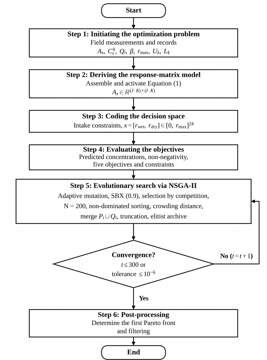
The five-objective optimization problem is solved using the elitist non-dominated sorting algorithm NSGA-II Deb et al. [5], implemented via the gamultiobj solver in MATLAB R2022a operating on the response matrix in Eq. (1). NSGA-II is well appropriate to this problem because it generates a well-distributed Pareto front in a single run without target summing or the need for derivatives, and because its constrained dominance principle directly addresses the intake constraints in Eq. (13). The procedure consists of six steps as included in flow chart presented in Figure 4. Table 17 presents the main algorithm inputs.
The Mersenne Twister generator was initialized with seed 0, and the complete generator state is stored with the results. The front of 77 non-dominated points follows directly from the settings: a population of 200 and a Pareto fraction of 0.386 retaining 77 individuals; no post-hoc filtering or manual selection was applied at any stage. The constraints were supplied through the nonlinear-constraint interface of the solver, and the maximum constraint violation over the completely returned front is exactly zero. The search terminated on reaching the generation limit rather than on the convergence tolerance, after 60,001 function evaluations, with a final average crowding distance of 0.0166 and a spread of 0.0905.
Figure 4. Flowchart of the multi-objective water quality management methodology using the NSGA-II algorithm
Table 17. Inputs for the NSGA-II algorithm
|
Parameter |
Value |
|
Population size N |
200 |
|
Maximum number of generations Tmax. |
300 |
|
Tolerance δ |
1 × 10⁻⁶ |
|
Crossover |
SBX/0.9 |
|
Mutation |
Adaptive polynomial |
|
Selection |
Two-way competition (crowded comparison) |
|
Dimensions of decision vector |
24 (3 sources × 4 pollutants × 2 seasons) |
|
Upper bound for removal fraction rmax. |
0.8 per pollutant |
|
Seasonal weights (γwet, γdry) |
0.5, 0.5 |
|
Strict constraints at intakes in (mg/L) |
TDS ≤ 1000; BOD ≤ 6; NO3 ≤ 50 |
|
Phosphate PO4 in (mg/L) |
Quadratic penalty (Obj₅), limit 0.5 |
|
Random number generator |
Mersenne Twister, seed 0 |
|
Pareto fraction |
0.386 |
|
Constraint handling |
Nonlinear constraint interface (nonlcon) |
|
Function evaluations |
60,001 |
|
Stopping criterion triggered |
Maximum generations reached |
|
Maximum constraint violation |
0 |
6.1 Pareto front
The NSGA-II algorithm resulted in 77 optimal Pareto front solutions. The important result of the strict intake constraints is that each of the 77 solutions satisfied all strict intake constraints for TDS, BOD, and NO3 in both seasons, with zero exceedances in all cases. Therefore, strict compliance is not a criterion between solutions, but rather a certain property of the front; trade-offs occur between the remaining objectives. Table 18 gives the range statistics for each objective across the Pareto front.
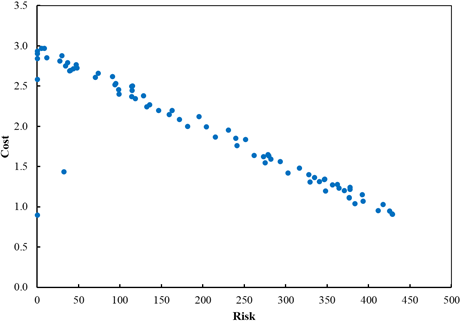
From the results in Table 18, it is obvious that the environmental risk extends from 0.154 to 429.97, while cost varies from 0.898 to 2.969. The frontier is governed by a high risk-cost contrast where cost increases accept substantial risk reductions in the low-cost zone, but produces diminishing returns as costs rise. Second, the intake water quality index (Obj3) takes a narrow range (-187.39 to -182.39). Because strict constraints are imposed on compliance by regulated components at intake, the resulting quality is high and relatively insensitive to the chosen solution. Thus, the real decision space is a trade-off between cost and residual risk, spatial equity, and phosphate control. Five representative solutions were obtained to characterize the front (Table 19): the lowest cost solution (No. 2), the lowest phosphate penalty solution (No. 77), the compromise solution (No. 31), the lowest risk solution (No. 4), and the best spatial justice solution (No. 3).
Table 18. Statistics for objectives across the optimal solutions on the Pareto front
|
Statistic |
Obj1 |
Obj2 |
Obj3 |
Obj4 |
Obj5 |
|
Minimum |
0.1542 |
0.898 |
-187.387 |
0.002 |
0.113 |
|
Median |
135.022 |
1.334 |
-186.993 |
11.839 |
0.117 |
|
Maximum |
429.965 |
2.969 |
-182.387 |
35.731 |
0.1443 |
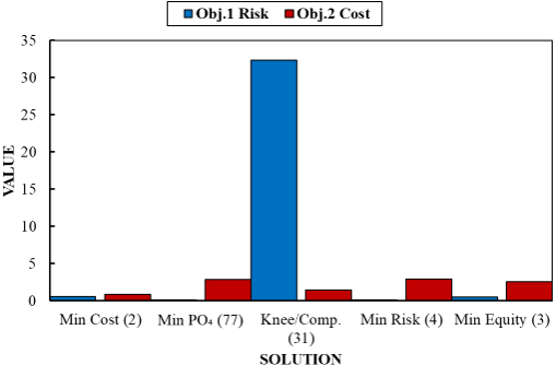
The five solutions reveal a fundamental conflict. Solution 2 achieves the lowest removal effort (0.898) at the highest residual risk among the four non-compromise representatives (0.543), while Solution 4 reaches the lowest risk (0.154) at a high cost (2.90). In descending order of Obj1 risk, the five representatives are No. 31 (32.3215), No. 2 (0.5430), No. 3 (0.4814), No. 77 (0.1719), and No. 4 (0.1542), so the compromise solution carries the highest risk of the five. Solution 77 minimizes the phosphate penalty (0.113) but again requires high costs (2.842). Solution 3 minimizes the variance of the residual exceedance load across the equity stations (Obj4 = 0.0022); this is the equity of the residual result and does not indicate an even distribution of treatment effort across the controllable sources. Solution 31 lies in the region of the risk-cost trade-off where marginal risk reduction begins to diminish, at (risk 32.32, effort 1.436). Solution 31 is identified here as the compromise solution of the front. Four independent criteria, two based on distance to reference points [19] and two on the geometry of the front [20], were applied to the complete front of 77 solutions, and all four are reported here, whether or not they agree. The five objectives were first scaled to the unit interval by min-max normalization over the front, since they differ in dimension and range by up to three orders of magnitude; the sensitivity of the outcome to that normalization was then tested by repeating the calculation with max-absolute scaling in place of min–max normalization (see Table 20).
Table 19. Results of the trade-offs between objectives
|
Solution Type |
Solution Number |
Obj1 |
Obj2 |
Obj3 |
Obj4 |
Obj5 |
|
Minimum cost |
2 |
0.543 |
0.898 |
-185.102 |
0.0067 |
0.1422 |
|
Minimum PO4 Penalty |
77 |
0.171 |
2.841 |
-187.387 |
0.0047 |
0.1130 |
|
Compromise |
31 |
32.32 |
1.435 |
-187.045 |
3.3535 |
0.1165 |
|
Minimum risk |
4 |
0.154 |
2.899 |
-187.351 |
0.0040 |
0.1134 |
|
Minimum spatial equity |
3 |
0.481 |
2.582 |
-186.639 |
0.0022 |
0.1211 |
Table 20. Selection criteria applied to the full Pareto front and the solution each one selects
|
Selection Criterion |
Definition |
Solution Selected |
|
Minimum distance to the ideal point |
Smallest Euclidean norm of the min-max normalized objective vector. |
31 |
|
TOPSIS closeness, equal weights |
Largest ratio of distance-to-nadir over the sum of both distances. |
31 |
|
Ideal-point distance with max-absolute scaling |
As above, objectives scaled only by their largest absolute value. |
31 |
|
Maximum curvature |
Largest local curvature of the Obj1-Obj2 projection. |
36 |
|
Maximum bend from the extreme chord |
Largest perpendicular offset from the line joining the two end points of the Obj1-Obj2 projection. |
2 |
Table 21. Position of Solution 31 within the front, by objective
|
Objective |
Value |
Normalized Position |
Rank among 77 by This Objective Alone |
|
Obj1 environmental risk |
32.3215 |
0.075 |
22 |
|
Obj2 removal effort |
1.4358 |
0.260 |
53 |
|
Obj3 intake quality index |
−187.045 |
0.069 |
30 |
|
Obj4 spatial equity |
3.3535 |
0.094 |
22 |
|
Obj5 phosphate penalty |
0.1166 |
0.114 |
30 |
Three of the four criteria select Solution 31, and this selection is unchanged when min–max normalization is replaced by max-absolute scaling. Solution 31 is therefore the compromise solution of the front; it is not the knee in the geometric sense, which the curvature-based criteria place at Solutions 36 and 2. The two curvature-based criteria disagree with each other and with the rest, and the reason is instructive rather than troubling: both operate on the two-dimensional Obj1-Obj2 projection and are therefore blind to the remaining three objectives. Maximum curvature selects Solution 36, which ranks nineteenth by distance to the ideal point and carries almost three times the environmental risk of Solution 31 for a similar removal effort. Maximum bend selects Solution 2, the extreme lowest-effort point, which ranks sixtieth of 77; this is a known failure of the chord method when one end of the front is far more densely populated than the other. Neither result recommends a different compromise solution; both show why a criterion defined across all five objectives is appropriate for a five-objective problem.
In normalized terms, it lies at 0.075 of the risk range and 0.260 of the cost range, securing most of the achievable risk reduction for about a quarter of the reached cost increase, while satisfying the TDS, BOD, and NO3 intake limits in full. It is therefore presented as a preliminary model-based reference scenario, pending the validation described in Section 3.4, rather than as an operational direction (See Table 21).
Figure 5. Comparison of the risk objective (Obj1) with the cost objective (Obj2) for the five representative solutions
Figure 6. Pareto front for Obj1 (risk) versus Obj2 (cost)
The margin is narrow, with Solution 31 leading Solution 63 by 0.019 in normalized distance, or six per cent of its own distance, and no other solution lies within five per cent of the best value. The four nearest alternatives occupy the same region of the front, with risk between 16 and 39 and effort between 1.43 and 1.59, so the choice among them is a matter of preference rather than of dominance. Solution 31 is accordingly presented as a preliminary model-based reference scenario, pending the validation described in Section 3.4, identified by an explicit and reproducible rule, and not as the unique optimum. Figure 5 relates the risk and cost values for the five representative solutions. Figure 6 shows the full Pareto front for the 77 solutions, showing the inverse relationship between risk, cost, and the position of the compromise solution near (32, 1.44); the position is determined in this section.
6.2 Intake compliance
Table 22 presents the predicted intake concentrations and the phosphate exceedance for all five representative solutions in both seasons.
TDS, BOD, and NO3 show zero exceedance at both intakes in both seasons in all five solutions, and the strict limits hold exactly as designed. The only constant exceedance is phosphate, which stays above the 0.5 mg/L target at both intakes throughout the dry season, with residues of 0.199 to 0.313 mg/L at Kufa and 0.432 mg/L at Al-Manadhira. The Al-Manadhira value is equal in all five solution points to a physical rather than an economic bound, and it alone accounts for 0.093 of the front-wide minimum of 0.113 in Obj5. Re-computing Obj5 independently from these residues through Eq. (12) produces the tabulated objective to four decimal places for every solution, which shows that the objective values, the intake concentrations, and the stated formulation are mutually consistent.
Table 22. Predicted intake concentrations and phosphate exceedances (mg/L) for the five representative solutions
|
Solution |
Season |
Intake |
TDS |
BOD |
NO3 |
PO4 |
PO4 Exceedance |
|
2 |
Dry |
Kufa |
884.5 |
2.090 |
0.317 |
0.813 |
0.313 |
|
Al-Manadhira |
888.2 |
1.492 |
-1.241 |
0.932 |
0.432 |
||
|
Wet |
Kufa |
952.8 |
4.645 |
0.617 |
-2.911 |
0 |
|
|
Al-Manadhira |
669.5 |
2.987 |
-1.063 |
-0.263 |
0 |
||
|
3 |
Dry |
Kufa |
875.7 |
2.045 |
-1.149 |
0.736 |
0.236 |
|
Al-Manadhira |
832.8 |
1.483 |
-2.076 |
0.932 |
0.432 |
||
|
Wet |
Kufa |
916.4 |
4.636 |
-1.155 |
-0.942 |
0 |
|
|
Al-Manadhira |
359.8 |
2.750 |
-8.210 |
0.025 |
0 |
||
|
4 |
Dry |
Kufa |
872.2 |
2.057 |
-0.282 |
0.701 |
0.201 |
|
Al-Manadhira |
811.2 |
1.485 |
-1.582 |
0.932 |
0.432 |
||
|
Wet |
Kufa |
906.5 |
4.638 |
-3.036 |
-11.15 |
0 |
|
|
Al-Manadhira |
300.7 |
2.588 |
-12.85 |
-4.790 |
0 |
||
|
31 |
Dry |
Kufa |
880.7 |
2.093 |
0.552 |
0.716 |
0.216 |
|
Al-Manadhira |
864.3 |
1.493 |
-1.107 |
0.932 |
0.432 |
||
|
Wet |
Kufa |
981.4 |
4.644 |
-0.599 |
-3.113 |
0 |
|
|
Al-Manadhira |
892.2 |
2.857 |
-3.673 |
-0.516 |
0 |
||
|
77 |
Dry |
Kufa |
872.1 |
2.057 |
-0.704 |
0.699 |
0.199 |
|
Al-Manadhira |
810.4 |
1.485 |
-1.822 |
0.932 |
0.432 |
||
|
Wet |
Kufa |
910.9 |
4.637 |
-2.605 |
-7.477 |
0 |
|
|
Al-Manadhira |
337.1 |
2.573 |
-10.82 |
-3.068 |
0 |
Note: TDS: Total Dissolved Solids; BOD: Biochemical Oxygen Demand.
Several nitrate and phosphate records in Table 16 are negative because the linear form C = C0-Ar yields a negative value whenever the attributed removal exceeds the baseline concentration, so their presence illustrates that the projection [C←max(0, C)] was applied when the constraints were evaluated but not to the reported concentration field. They are retained because they define the valid range of the response matrix, and because every one of them falls where the parameter lies far below its limit, so no compliance decision reported here depends on them.
6.3 Optimal removal tables
Table 23 lists the optimal removal ratios r*(i, k, s) at the controllable sources S3, S4, and S5 for the representative solutions.
Table 24 presents the seasonal comparison by parameter, counting the source-parameter pairs in which the dry-season ratio exceeds the wet-season ratio across all sixty pairs of Table 19.
Table 23. Optimal removal ratios at the controllable sources for the five representative solutions
|
Solution |
Pollutant |
Dry |
Wet |
||||
|
S3 |
S4 |
S5 |
S3 |
S4 |
S5 |
||
|
2 |
TDS |
0.249 |
0.176 |
0.060 |
0.283 |
0.324 |
0.197 |
|
BOD |
0.092 |
0.407 |
0.392 |
0.464 |
0.160 |
0.012 |
|
|
PO4 |
0.166 |
0.285 |
0.190 |
0.421 |
0.182 |
0.016 |
|
|
NO3 |
0.535 |
0.548 |
0.015 |
0.204 |
0.350 |
0.044 |
|
|
3 |
TDS |
0.285 |
0.306 |
0.446 |
0.184 |
0.525 |
0.611 |
|
BOD |
0.684 |
0.535 |
0.585 |
0.624 |
0.666 |
0.213 |
|
|
PO4 |
0.406 |
0.753 |
0.663 |
0.080 |
0.117 |
0.151 |
|
|
NO3 |
0.427 |
0.564 |
0.530 |
0.239 |
0.370 |
0.428 |
|
|
4 |
TDS |
0.493 |
0.389 |
0.371 |
0.417 |
0.569 |
0.476 |
|
BOD |
0.460 |
0.424 |
0.669 |
0.424 |
0.535 |
0.350 |
|
|
PO4 |
0.770 |
0.800 |
0.800 |
0.676 |
0.773 |
0.304 |
|
|
NO3 |
0.343 |
0.586 |
0.342 |
0.401 |
0.486 |
0.617 |
|
|
31 |
TDS |
0.371 |
0.201 |
0.151 |
0.165 |
0.141 |
0.093 |
|
BOD |
0.144 |
0.280 |
0.423 |
0.429 |
0.168 |
0.122 |
|
|
PO4 |
0.770 |
0.722 |
0.643 |
0.357 |
0.230 |
0.060 |
|
|
NO3 |
0.402 |
0.519 |
0.109 |
0.317 |
0.446 |
0.137 |
|
|
77 |
TDS |
0.503 |
0.395 |
0.363 |
0.441 |
0.488 |
0.469 |
|
BOD |
0.479 |
0.408 |
0.677 |
0.516 |
0.568 |
0.363 |
|
|
PO4 |
0.800 |
0.800 |
0.798 |
0.558 |
0.437 |
0.252 |
|
|
NO3 |
0.384 |
0.587 |
0.422 |
0.404 |
0.491 |
0.502 |
|
Note: TDS: Total Dissolved Solids; BOD: Biochemical Oxygen Demand.
Table 24. Seasonal comparison of the optimal removal ratios by parameter
|
Parameter |
Number of Dry > Wet Pairs |
Out of |
Percentage |
|
TDS |
6 |
15 |
40.0% |
|
BOD |
9 |
15 |
60.0% |
|
PO4 |
14 |
15 |
93.3% |
|
NO3 |
9 |
15 |
60.0% |
|
All parameters |
38 |
60 |
63.3% |
Note: TDS: Total Dissolved Solids; BOD: Biochemical Oxygen Demand.
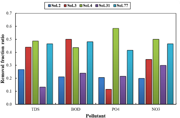
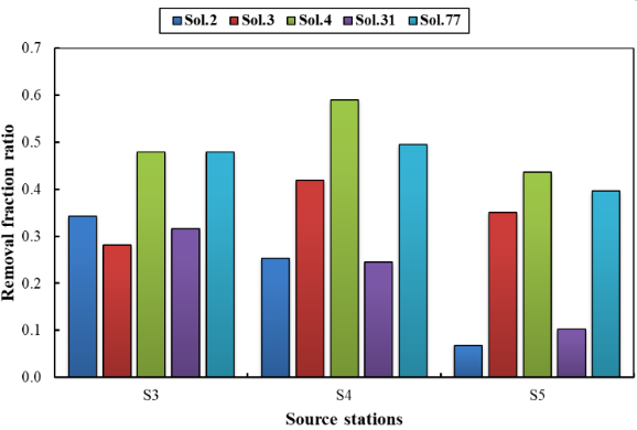
Figure 7. Variation of removal fraction ratios per pollutant for wet and dry seasons
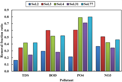
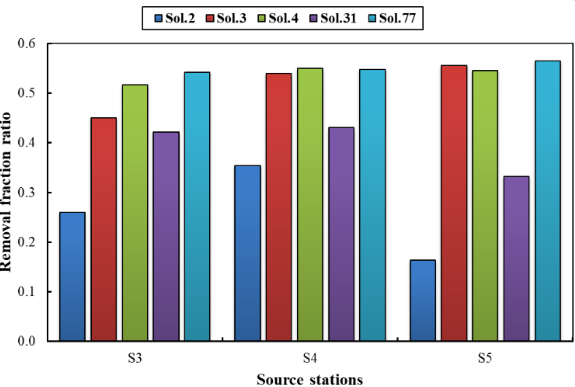
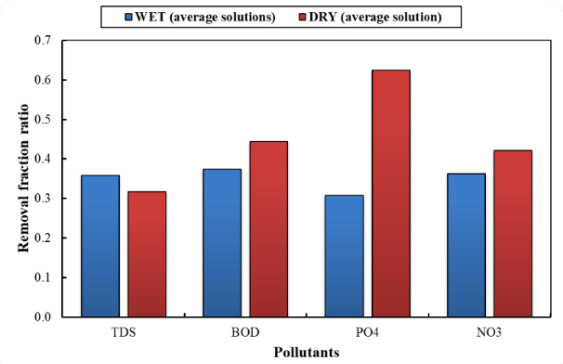
Three main patterns emerge. First, removal effort is higher in the dry season for most parameters. Across the 60 paired dry–wet comparisons in Table 23 (five solutions × three sources × four parameters), the dry-season ratio exceeds the wet-season ratio in 38 cases (63.3%; Table 24), and for PO4 in 14 of 15. The pattern follows the dilution deficit. Although the wet-season baselines at the three controllable sources exceed the dry-season values by factors of 1.26 for TDS, 5.09 for BOD, 1.86 for NO3, and 4.31 for PO4, the reduced dry-season discharge concentrates whatever load remains, so a larger fraction must be removed to hold the same concentration at the intakes. PO4 shows this most severely, with its dry-season removal reaching the feasible bound at all three sources in the low-phosphate solutions. Second, the low-risk solutions (No. 4 and No. 77) distribute removal comparatively evenly across the three sources, Solution 4 spanning 0.304 to 0.800 and Solution 77 covering 0.252 to 0.800, consistent with sustained operation of three treatment points; the compromise solution (No. 31) instead shows an irregular longitudinal pattern, with high NO3 removal at S3 and S4 but an obvious drop at S5, which explains its higher risk value. Third, PO4 control is limited by treatment capacity rather than priority: the algorithm applies the maximum feasible removal, and the remaining residue is a physical limit of the dry-season regime. Figures 7, 8 and 9 show the behavior of the optimal removal ratios by parameter and by source.
Figure 7 shows the variation in removal ratios according to the component for the wet and dry seasons; Figure 8 shows their variation according to the source stations (S3, S4, S5), and Figure 9 compares the removal ratios by parameter between the two seasons, resolving the seasonal comparison by parameter and by source rather than attributing it to dilution alone.
Figure 8. Variation of removal fraction ratios per source station for wet and dry seasons
Table 25. Comparison of the two constraint scenarios
|
Criterion |
Scenario 1* |
Scenario 2** |
Change |
|
Scope of the hard constraints |
Kufa and Al-Manadhira intakes |
All river stations S1 to S7, in both seasons |
- |
|
Constrained parameters |
TDS 1000, BOD 6, NO3 50 mg/L |
TDS 1000, BOD 6, NO3 50 mg/L |
Unchanged |
|
Phosphate |
Penalty objective at the intakes, 0.5 mg/L |
Penalty objective at the intakes, 0.5 mg/L |
Unchanged |
|
Controllable sources |
S3, S4, S5 |
S3, S4, S5 |
Unchanged |
|
Decision-vector dimension |
24 |
24 |
Unchanged |
|
Points on the Pareto front |
77 |
77 |
Unchanged |
|
Solutions satisfying the constraints |
77 (100%) |
13 (16.9%) |
-83.1% |
|
Compromise solution |
No. 31 |
No. 35 |
Changed |
|
Obj1 (compromise solution) |
32.32 |
0.161 |
-99.5% |
|
Obj2 (compromise solution) |
1.436 |
2.099 |
+46.2% |
|
Obj3 (compromise solution) |
-187.045 |
-187.256 |
-0.1% |
|
Obj4 (compromise solution) |
3.354 |
0.00426 |
-99.9% |
|
Obj5 (compromise solution) |
0.1165 |
0.1144 |
-1.8% |
|
Dry-season PO4 residue at Al-Manadhira (mg/L) |
0.432 |
0.432 |
Unchanged |
Note: *constraints at the intakes; **constraints at all stations.
6.4 Sensitivity of the Pareto set to the range of the constraints
The problem was re-solved with the IQS limits enforced not at the two intakes alone but at all seven river stations in both seasons, the controllable sources, the decision vector, and the objective set being left unchanged. Because the front itself is generated from the same data, the 77 non-dominated points are common to both runs, and the scenarios differ only in which of them survive the feasibility test. Table 25 sets out the comparison.
The effect is substantial, applying the limits at every station reduces the admissible set from all 77 solutions to 13, or 16.9%, and moves the compromise solution from No. 31 to No. 35. The reference plan changes nature with it: environmental risk falls from 32.32 to 0.161 and the variance of the residual exceedance load falls from 3.354 to 0.00426, while the removal effort rises by 46%, from 1.436 to 2.099. The intake water quality index and the phosphate penalty improve only marginally, and the dry-season PO4 residue at Al-Manadhira remains at 0.432 mg/L in both scenarios, which is further evidence that this residue is physically bound rather than a consequence of the constraint set. Scenario (2) therefore achieves a near-complete elimination of in-river risk and a nearly uniform distribution of treatment for a little under half as much effort, and the choice between the two is a scheme question rather than a computational one.
Figure 9. Comparison between removal fraction ratios per pollutant for wet and dry seasons
This study presents a novel methodology to formulate and solve the case of strict intake constraints for managing the Kufa River under multiple flow regimes, combining the MIKE 11 hydrodynamic model and calibrated water quality with a seasonal linear response-matrix model and the NSGA-II. The main conclusions are as follows.
1. A coupled simulation-optimization methodology that distinguishes strictly applied intake constraints from penalty components is well posed and, on the present evidence, practically solvable for the Kufa River. All 77 Pareto-optimal solutions satisfied the IQS limits for TDS, BOD, and NO3 at the Kufa and Manadhira intakes with zero exceedance in both wet and dry seasons.
2. The Pareto front is governed by a sharp environmental risk conflict (risk 0.154–429.97 versus cost 0.898-2.969), while the intake water quality index remains high and narrow-ranged because strict compliance is ensured. The compromise solution (No. 31; cost 1.436) is selected by minimum normalized distance to the ideal point and is supported by equal-weight TOPSIS and remains unchanged when min–max normalization is replaced by max-absolute scaling; it is presented as a preliminary model-based reference scenario, pending the validation described in Section 3.4, rather than as an operating policy, surrounded by the lowest-cost (No. 2) and minimum-phosphate (No. 77) solutions.
3. Phosphate is the dominant stress on the system water quality and reveals strong seasonal asymmetry: wet-season dilution eliminates intake exceedances, while dry-season residues of 0.20–0.43 mg/L above the 0.5 mg/L target persist at the intakes even under the maximum feasible removal, most significantly at the downstream Al-Manadhira intake, where the residual of 0.432 mg/L cannot be eliminated by any permissible removal schedule.
4. This physical limit justifies the penalty treatment of phosphate, which preserves a feasible front that a strict PO4 constraint would have rendered empty.
5. Removal effort is higher in the dry season, in 38 of the 60 paired dry–wet comparisons and in 14 of 15 for PO4, because reduced dilution concentrates the residual load at the intakes. The low-risk solutions reach relatively balanced removal across S3 to S5, while the compromise solution is retained mainly for its risk-effort balance despite its less consistent allocation.
6. The practical quality of the optimized solutions remains limited by modelling uncertainty. In particular, TDS at the Kufa intake represents the critical constraint, while the deterministic optimization, average hydrodynamic calibration performance, and existing treatment-capacity limitations reveal the need for uncertainty analysis and site-specific feasibility assessment.
[1] Khair-Allah, Z.H., Khassaf, S.I. (2026). Impact of climate change and upstream development on domestic water security in the Euphrates River Basin, Iraq. Iraqi Geological Journal, 59(1B). https://doi.org/10.46717/igj.2026.59.1B.2
[2] UN-ESCWA, BGR (United Nations Economic and Social Commission for Western Asia, Bundesanstalt für Geowissenschaften und Rohstoffe). (2013). Inventory of Shared Water Resources in Western Asia. UN-ESCWA and BGR, Beirut, Lebanon. https://digitallibrary.un.org/record/790315?v=pdf.
[3] Burn, D.H., Yulianti, J.S. (2001). Waste-load allocation using genetic algorithms. Journal of Water Resources Planning and Management, 127(2): 121-129. https://doi.org/10.1061/(ASCE)0733-9496(2001)127:2(121)
[4] Nicklow, J., Reed, P., Savic, D., et al. (2010). State of the art for genetic algorithms and beyond in water resources planning and management. Journal of Water Resources Planning and Management, 136: 412-432. https://doi.org/10.1061/(ASCE)WR.1943-5452.0000053
[5] Deb, K., Pratap, A., Agarwal, S., Meyarivan, T. (2002). A fast and elitist multiobjective genetic algorithm: NSGA-II. IEEE Transactions on Evolutionary Computation, 6(2): 182-197. https://doi.org/10.1109/4235.996017
[6] Arora, J.S. (2004). Introduction to Optimum Design. Elsevier.
[7] Garcia, J.A., Alamanos, A. (2024). Optimization in water resources management. In Elgar Encyclopedia of Water Policy, Economics and Management, Edward Elgar Publishing, pp. 188-191. https://doi.org/10.4337/9781802202946.00050
[8] Allam, A., Tawfik, A., Yoshimura, C., Fleifle, A. (2016). Multi-objective models of waste load allocation toward a sustainable reuse of drainage water in irrigation. Environmental Science and Pollution Research, 23: 13026-13038. https://doi.org/10.1007/s11356-016-6331-z
[9] DHI, D. (2003). Mike-11: A modelling system for rivers and channels, reference manual. DHI-Water and Development, Horsholm, Denmark.
[10] COQS (2009) Iraqi Standard of Drinking Water No. 417. Second Modification, Central Organization for Quality Control and Standardization, Council of Ministers, Baghdad.
[11] Kareem, H.H., Alkatib, A.A. (2022). Future short-term estimation of flowrate of the Euphrates River catchment located in Al-Najaf Governorate, Iraq through using weather data and statistical downscaling model. Open Engineering, 12(1): 129-141. https://doi.org/10.1515/eng-2022-0027
[12] Kashkool, M.J., Obead, I.H. (2025). Assessment of pollution risks in the Kufa River using water quality indices and principal component analysis. International Journal of Design & Nature and Ecodynamics, 20(4): 737-752. https://doi.org/10.18280/ijdne.200405
[13] Kashkool, M.J., Obead, I.H. (2026). Hydrodynamic and pollutant distribution in the Euphrates River under the impact of extreme flow conditions using numerical analysis and parameter calibration. Ecological Engineering & Environmental Technology, 27(2): 33-45. https://doi.org/10.12912/27197050/215873
[14] Moriasi, D.N., Arnold, J.G., Van Liew, M.W., Bingner, R.L., Harmel, R.D., Veith, T.L. (2007). Model evaluation guidelines for systematic quantification of accuracy in watershed simulations. Transactions of the ASABE, 50(3): 885-900. https://doi.org/10.13031/2013.23153
[15] Irvine, D.J., Werner, A.D., Ye, Y., Jazayeri, A. (2021). Upstream dispersion in solute transport models: A simple evaluation and reduction methodology. Groundwater, 59: 287-291. https://doi.org/10.1111/gwat.13036
[16] Chernysh, Y., Stejskalová, L., Soldán, P., et al. (2025). Risk assessment as a tool to improve water resource management. Water Resources Management, 39(1): 47-63. https://doi.org/10.1007/s11269-024-03982-x
[17] Shokoohi, M., Tabesh, M., Nazif, S., Dini, M. (2017). Water quality based multi-objective optimal design of water distribution systems. Water Resources Management, 31: 91-108. https://doi.org/10.1007/s11269-016-1512-6
[18] Crini, N., Lichtfouse, E., Fourmentin, M., et al. (2022). Removal of emerging contaminants from wastewater using advanced treatments: A review. Environmental Chemistry Letters, 20: 1333-1375. https://doi.org/10.1007/s10311-021-01379-5
[19] Hwang, C.L., Yoon, K. (1981). Multiple Attribute Decision Making: Methods and Applications. Springer, Berlin, Heidelberg. https://doi.org/10.1007/978-3-642-48318-9
[20] Das, I. (1999). On characterizing the “knee” of the Pareto curve based on normal-boundary intersection. Structural Optimization, 18(2-3): 107-115. https://doi.org/10.1007/BF01195985