Mohammad Azis Mahardika* | Agus Hermanto | Diki Ismail Permana | Rozaan Faros Al Ihsan
© 2026 The authors. This article is published by IIETA and is licensed under the CC BY 4.0 license (http://creativecommons.org/licenses/by/4.0/).
OPEN ACCESS
Static mixers are employed to enhance fluid homogenization under laminar flow conditions, where mixing depends primarily on repeated flow splitting, stretching, folding, and radial redistribution rather than turbulent fluctuations. This study investigates the effect of element cross-sectional branching on the balance between mixing uniformity and hydraulic resistance of twisted static mixers at low Reynolds numbers (Re). Three element configurations were examined: conventional I-shaped, Y-shaped, and cross-shaped twisted elements. Simulations were performed for Re ranging from 50 to 1000 using water and sodium chloride solution. Mixing uniformity was quantified using the coefficient of variation (CoV), whereas hydraulic resistance was characterized through the friction factor. The results demonstrate that the element cross-section influences the trade-off between mixing effectiveness and pressure loss. The I-shaped mixer generated the lowest friction factor but exhibited the highest CoV, indicating insufficient tracer redistribution. The Y-shaped element enhanced flow division and radial transport, thereby improving mixing with a moderate increase in hydraulic resistance. The cross-shaped mixer achieved the best uniformity, with coefficient-of-variation values of approximately 0.04–0.11, but it produced the highest friction factor due to greater blockage. Therefore, the optimal static mixer geometry depends on the required outlet uniformity and the allowable pumping cost, rather than on a single universal best configuration.
static mixer, cross-sectional shape, coefficient of variation, friction factor, computational fluid dynamics
Static mixers are widely used in chemical [1], environmental [2], water treatment [3], food, and process industries [4, 5] because they enhance fluid mixing without moving mechanical components. Compared with mechanically agitated systems, static mixers offer several advantages, including compact construction, simple operation, low maintenance requirements, and suitability for continuous inline processes [6]. Mixing is generated between the static mixer inside the tube and the flowing fluid. It modifies the flow pattern by dividing, rotating, stretching, and redistributing the fluid streams along the pipe's axial direction [7].
Among various static mixer designs, the Kenics-type static mixer is one of the most commonly studied configurations [8]. The conventional Kenics static mixer consists of a series of twisted elements, where each element is typically rotated to give helices with a 180° twist of a determined length. This arrangement promotes repeated flow division and radial redistribution, making it effective for laminar mixing applications. In low Reynolds number (Re) flows, where turbulence is absent or limited, mixing relies mainly on split, redirect, and recombine flow due to stationary elements [9]. Therefore, the geometry of the mixing element is a critical factor in determining mixing performance.
At low Re, both dispersive and distributive mixing are enhanced by helical mixing, and an increase in Re can improve dispersive and distributive mixing [10]. However, the relationship between Re and mixing quality is not always linear, because higher velocity also reduces the residence time available for diffusion and can alter the internal flow structure [11]. As a result, an optimum operating range may exist where the balance between flow deformation and residence time produces the best mixing uniformity.
Previous studies have shown that the mixing behavior of Kenics-type static mixers is strongly influenced by Re, number of elements, element aspect ratio, twist direction, and pressure drop characteristics [9, 12-14].
Other studies have attempted to reduce the pressure-drop penalty by introducing gaps between Kenics elements, while maintaining acceptable mixing performance [15]. Element thickness has also been investigated because it affects blockage, pressure drop, mixing performance, and friction factor [16]. These studies indicate that the performance of a static mixer is generally evaluated using both mixing indicators, such as coefficient of variation (CoV), and hydraulic indicators, such as pressure drop or friction factor.
In addition to conventional Kenics mixers, recent studies have proposed new static mixer configurations, such as curved-sheet blade-folded mixers and symmetrical folded-blade mixers, to improve flow redistribution and enhance mixing performance [17]. These developments show that the internal geometry of the mixing element strongly affects the flow field, radial transport, and mixing uniformity [18]. However, most existing studies still focus on modifying the aspect ratio, spacing, thickness, blade shape, or commercial mixer configurations. The direct effect of element cross-sectional branching in a twisted static mixer remains less clearly discussed.
Due to the complex geometry of the Kenics static mixer, analytical studies cannot be used. Computational fluid dynamics (CFD) has been used to simulate the Kenics static mixer and provides insight into the mixing mechanism [16, 19, 20].
The investigation of I-shaped, Y-shaped, and cross-shaped twisted elements is therefore important because these geometries represent different levels of flow-path branching. The conventional I-shaped element mainly divides the flow into two dominant passages, whereas the Y-shaped and cross-shaped elements introduce three and four branches, respectively. Under laminar flow conditions, where turbulence is absent, mixing depends strongly on the ability of the mixer to split, stretch, fold, and redistribute the fluid across the pipe cross-section. Increasing the number of branches is expected to enhance radial redistribution and scalar stretching, thereby improving concentration uniformity. However, the same geometric modification may also increase blockage, wetted surface area, local velocity gradients, and pressure drop.
Therefore, the present study differs from previous research on Kenics static mixers by isolating the effect of element cross-sectional shape while keeping the pipe diameter, number of elements, twist angle, and operating conditions identical. The I-shaped geometry is used as the conventional reference, while the Y-shaped and cross-shaped geometries are evaluated as branched-element modifications. The main contribution of this work is to clarify how cross-sectional branching affects the trade-off between mixing uniformity, represented by the CoV, and hydraulic resistance, represented by the friction factor.
2.1 Physical model and fluid properties
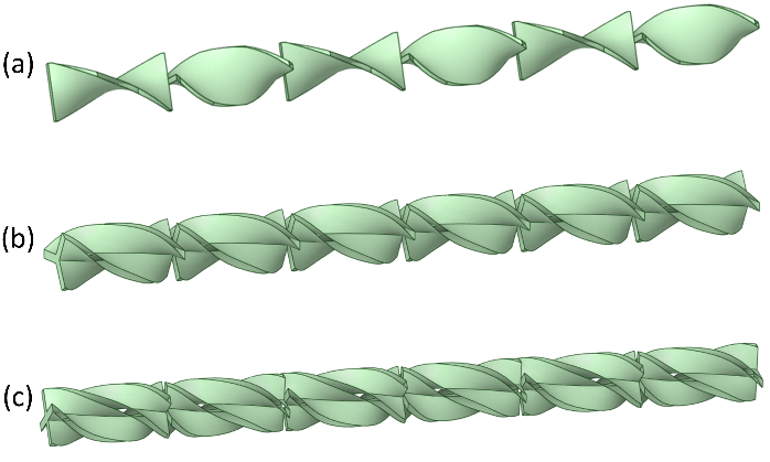
This study investigates the mixing performance of three twisted static mixer configurations, namely an I-shaped, a Y-shaped, and cross-shaped. The I-shaped is used as the reference geometry because it represents the conventional Kenics-type twisted element. The Y-shaped and cross-shaped geometries are proposed as modified geometries in which the cross-sectional shape of the twisted element is changed to increase the number of flow-splitting branches, as shown in Figure 1.
Figure 1. Static mixer geometries: (a) I-shaped, (b) Y-shaped, and (c) cross-shaped
The static mixer was designed with six twisted elements to provide repeated flow splitting, rotation, and recombination along the pipe. This number of elements was selected as a compromise between mixing development and computational cost. A smaller number of elements may not provide sufficient repeated redistribution to evaluate the mixing mechanism. In contrast, a much larger number of elements would increase computational demand without changing the main objective of this study, which is to compare the influence of element cross-sectional shape.
Each element was designed with a 180° twist angle. This angle was selected because it represents the conventional Kenics-type twisted element and provides a common baseline for evaluating the modified cross-sectional geometries. By maintaining the same twist angle for all configurations, the effect of twisting was kept constant, allowing the influence of cross-sectional shape to be evaluated more directly.
The same pipe diameter, element length, number of elements, twist angle, inlet condition, outlet condition, and fluid properties were used for the I-shaped, Y-shaped, and cross-shaped mixers. This approach was adopted to isolate the effect of element cross-sectional shape on mixing performance and hydraulic resistance. Therefore, any difference between CoV and the friction factor can be mainly attributed to changes in element geometry rather than to differences in mixer dimensions or operating conditions.
All mixer configurations are placed inside a circular pipe with a diameter of 21 mm and an aspect ratio of 2, containing 6 elements. Each mixer element is twisted 180°.
In the present study, steady laminar flow was assumed to enable a controlled comparison of the three static mixer geometries. The main objective is to evaluate the effect of the element's cross-sectional shape. Under laminar conditions, mixing in a static mixer is mainly governed by flow splitting, stretching, folding, and radial redistribution rather than by turbulent fluctuations. Therefore, the steady laminar formulation is considered suitable for evaluating the relative geometry-driven mixing behavior of the proposed configurations.
Table 1. Properties of the fluids
|
Parameter |
Water |
Brine |
|
Density (kg/m3) |
998.2 |
998.2 |
|
Viscosity (kg/m.s) |
0.001 |
0.001 |
|
Diffusion coefficient (m2/s) |
1.44 × 10⁻⁹ |
1.44 × 10⁻⁹ |
|
Reynolds number (Re) |
50-1000 |
50-1000 |
The working fluids in the simulation are water and brine (NaCl solution); detailed properties of these fluids are set out in Table 1. The brine is assumed to have the same density and viscosity as water to isolate the effect of mixer geometry. This assumption was intentionally applied to isolate the effect of mixer geometry on concentration redistribution. By neglecting density and viscosity differences between the two miscible streams, additional effects such as buoyancy-driven motion, viscosity-induced stratification, and property-dependent flow distortion were avoided. As a result, the predicted concentration field represents the influence of the internal mixer structure on convective transport and distributive mixing. This assumption is appropriate for a comparative numerical study in which the main focus is the influence of the element's cross-sectional shape rather than the effect of the fluid-property contrast. The physical properties of the working fluid are kept constant for all simulation cases.
2.2 Governing equations and numerical details
The flow is assumed to be three-dimensional, steady, incompressible, and laminar. The governing equations consist of the continuity, momentum, and species transport equations. These equations are solved using the finite volume method.
The continuity equation is expressed as Eq. (1):
$\nabla .(\rho V)=0$ (1)
The momentum equation is expressed as Eq. (2):
$\nabla \cdot(\rho V V)=-\nabla P+\nabla \cdot[\mu \nabla V]+\rho g$ (2)
The species transport equation is expressed as Eq. (3):
$\nabla \cdot\left(\rho V Y_A\right)=\nabla \cdot\left(\rho D_{A B} \nabla Y_A\right)$ (3)
where, ρ is the fluid density, V is the velocity vector, P is the pressure, μ is the dynamic viscosity, YA is the mass fraction of the tracer, and DAB is the molecular diffusion coefficient.
The pressure-velocity coupling is solved using the SIMPLE algorithm. The convective terms in the momentum and species transport equations are discretised using a second-order upwind scheme to reduce numerical diffusion. The convergence criterion is set to residuals below 10-5. ANSYS Fluent software was used to solve the numerical simulation
2.3 Boundary conditions
The Re is used to define the flow condition inside the static mixer and is calculated as Eq. (4):
$\operatorname{Re}=\rho V D / \mu$ (4)
where, Re is the Reynolds number, ρ is the fluid density, V is the average inlet velocity, D is the pipe diameter, and μ is the dynamic viscosity. The inlet velocity is adjusted to obtain the selected Re in the low Re range.
A velocity inlet boundary condition is applied at the inlet of the pipe. A pressure outlet boundary condition with zero gauge pressure is applied at the outlet. No-slip boundary conditions are applied to the pipe wall and all mixer element surfaces.
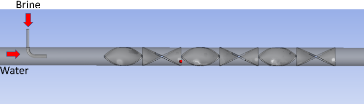
Figure 2. Static mixer inlet configuration
To evaluate mixing performance, brine is injected into the tube from the small pipe shown in Figure 2. This condition represents two initially unmixed miscible fluids entering the mixer. The same inlet concentration condition is used for all mixer configurations.
2.4 Grid independence test
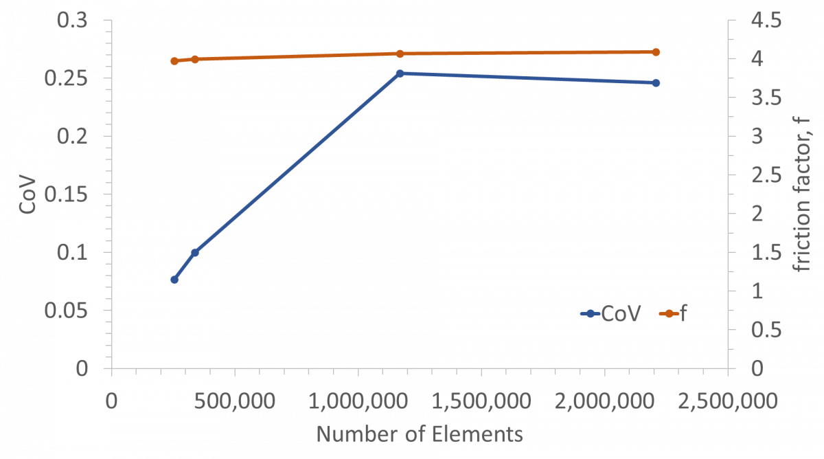
A grid independence test was performed to ensure that the numerical results were not significantly affected by mesh density. Several mesh sizes were evaluated by comparing the CoV and friction factor. These two parameters were selected because they represent the main performance indicators of the static mixer, namely mixing quality and hydraulic resistance.
The results of the grid independence test are shown in Figure 3. The CoV changes significantly when the mesh is increased from approximately 0.3 million to 1.2 million elements. However, further refinement from approximately 1.2 million to 2.3 million elements produces only a small change in CoV. A similar trend is observed for the friction factor, with the value remaining nearly constant over the tested mesh range. This indicates that the numerical solution becomes less sensitive to mesh refinement after approximately 1.2 million elements.
Figure 3. Grid independence test for Kenics static mixer, Reynolds numbers (Re) = 100
Therefore, the mesh with approximately 1.2 million elements, corresponding to a 1 mm mesh size, was selected for the final simulations. This mesh provides a reasonable balance between numerical accuracy and computational cost.
2.5 Model validation
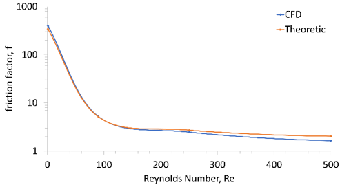
Model validation is conducted to ensure the reliability of the CFD method before applying it to the modified mixer geometries. In this study, the numerical model is validated using the friction factor. The friction factor obtained from the CFD simulation is compared with an available theoretical correlation for static mixer flow under the same Re range.
The Darcy friction factor is calculated as Eq. (5):
$f=2 \Delta P D /\left(\rho L V^2\right)$ (5)
where, f is the Darcy friction factor, ΔP is the pressure drop, D is the pipe diameter, ρ is the fluid density, L is the evaluated pipe length, and V is the average inlet velocity.
The correlations for calculating f in a Kenics static mixer [21] are shown in Eq. (6):
$f=\frac{342}{R e}+15$ (6)
As shown in Figure 4, the CFD results follow the same trend as the theoretical correlation for the friction factor. The friction factor decreases significantly with increasing Re, indicating that the numerical model is able to capture the expected flow-resistance behavior in the low Re range. The difference between the CFD and theoretical values becomes relatively small over the investigated Re range. Therefore, the CFD model is considered acceptable for further evaluation of the I-shaped, Y-shaped, and cross-shaped twisted static mixers.
Figure 4. Theoretical and computed computational fluid dynamics (CFD) friction factor for various Reynolds numbers (Re)
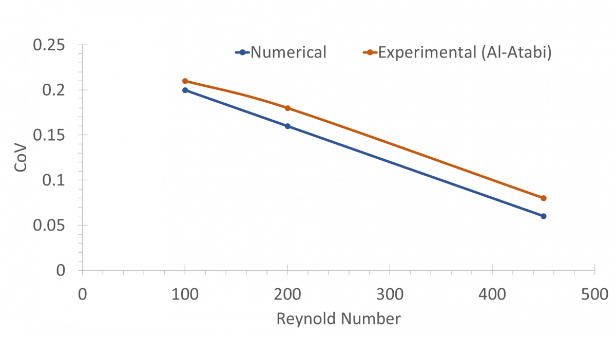
In addition to friction-factor validation, the predicted CoV was compared with the experimental data reported by Al-Atabi [22] because the study provides direct experimental measurements of mixing quality using the CoV for water-brine mixing in a baffled static mixer. As shown in Figure 5, the numerical results follow the same trend as the experimental data, with the CoV decreasing as the Re increases. This trend indicates that the CFD model can reasonably capture the improvement of mixing uniformity at higher Re. Therefore, the CoV comparison provides additional support for the predicted mixing performance behaviour.
Figure 5. Experimental and computed computational fluid dynamics (CFD) coefficient of variation (CoV) for various Reynolds numbers (Re)
2.6 Mixing performance evaluation
The CoV was used to quantify the degree of concentration non-uniformity at the mixer outlet. This parameter is calculated from the standard deviation of the scalar concentration divided by the mean concentration over the outlet plane. A lower CoV indicates a more uniform concentration distribution and, therefore, better mixing performance. CoV was selected because it provides a simple, dimensionless, and quantitative indicator for comparing the mixing quality of different mixer geometries under the same inlet concentration, outlet location, and operating conditions.
The CoV is calculated as Eq. (7):
$\operatorname{CoV}=\sqrt{\frac{\sum_{i=1}^N\left(Y_i-Y_{\text {mean }}\right)^2}{N-1}} \frac{1}{Y_{\text {mean }}}$ (7)
where, Yi is the local tracer mass fraction at the i-th sampling point, Ymean is the mean tracer mass fraction at the outlet cross-section, and N is the number of evaluation points.
The main advantage of using CoV is that it directly represents the statistical uniformity of the scalar field at a selected cross-section. Therefore, it is suitable for evaluating the relative performance of the I-shaped, Y-shaped, and cross-shaped static mixers. However, CoV also has limitations. It is a global outlet-based parameter and does not fully describe local concentration structures, scalar stretching history, or microscopic mixing. For this reason, the CoV results were interpreted alongside concentration contours, streamline patterns, and friction factors to provide a more complete explanation of the mixing mechanism and hydraulic penalty.
2.7 Pressure drop evaluation
Pressure drop is also evaluated because static mixers improve mixing by disturbing the flow, which may increase hydraulic resistance. The pressure drop is calculated as the area-weighted average of the pressure difference between the inlet and outlet sections.
The comparison of pressure drops among the three mixer configurations is used to determine the hydraulic resistance resulting from modifying the element cross-sectional shape. A good static mixer should provide a low CoV while maintaining an acceptable pressure drop.
The flow and mixing behavior of the I-shaped, Y-shaped, and cross-shaped twisted static mixers were evaluated using CFD simulation. The results are discussed in terms of the concentration and velocity distributions, the friction factor, and the CoV. The CoV was used as the main indicator of mixing quality, while the friction factor was used to evaluate the hydraulic resistance of each mixer configuration.
3.1 Concentration distribution at different mixing elements
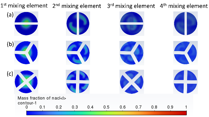
Figure 6 shows the tracer mass fraction distribution at different cross-sections along the mixer for the I-shaped, Y-shaped, and cross-shaped twisted static mixers at Re = 50. The concentration contours clearly show that the element cross-sectional shape affects the redistribution of the tracer inside the pipe.
Figure 6. Tracer mass fraction distribution at different cross-sections of the static mixers (Reynolds number (Re) = 50): (a) I-shaped, (b) Y-shaped, and (c) cross-shaped twisted static mixer
For the I-shaped mixer, the tracer is divided mainly into two regions due to the presence of the twisted flat plate. After the first mixing element, a high-concentration region remains near the central part of the cross-section. As the flow passes through the following elements, the tracer is gradually stretched and redistributed. However, the distribution is still relatively non-uniform even after the fourth mixing element. This indicates that the conventional I-shaped element provides limited flow division compared with the modified geometries.
For the Y-shaped mixer, the tracer distribution becomes more dispersed because the element divides the flow into three branches. The concentration field is stretched into several regions and distributed more effectively across the cross-section. Compared with the I-shaped mixer, the Y-shaped mixer shows better radial redistribution of tracer after each mixing element.
The cross-shaped mixer shows the most uniform concentration distribution among the three configurations. The four branches of the cross-shaped element divide the flow into more regions and promote stronger radial redistribution. After several mixing elements, the tracer concentration becomes more evenly distributed across the pipe section. This result indicates that increasing the number of twisted branches improves the distributive mixing mechanism.
Overall, the concentration distribution confirms that the cross-sectional shape of the twisted element significantly influences the mixing process. The cross-shaped mixer achieves the most effective tracer redistribution, followed by the Y-shaped and I-shaped mixers.
3.2 Flow redistribution and mixing mechanism
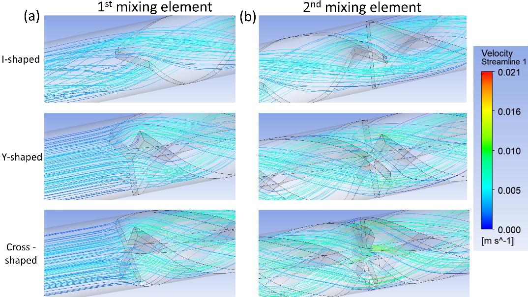
The streamline patterns in Figure 7 illustrate the flow redistribution mechanism generated by the twisted static mixer elements. As shown in Figure 7(a), the first mixing element initiates the deviation of the incoming axial flow. The streamlines are forced to move around the element surface, producing flow splitting and transverse displacement. This indicates that the incoming streams no longer move only in the axial direction, but begin to follow curved and helical trajectories. This mechanism is important for laminar mixing because, in the absence of turbulence, scalar homogenization mainly depends on repeated flow splitting, stretching, and radial redistribution.
The effect becomes more pronounced around the second mixing element, as shown in Figure 7(b). After passing through the first element, the flow entering the second element has already been displaced from its original position. The second element further redirects the streamlines and promotes recombination of previously separated flow paths. This repeated splitting–reorientation–recombination process increases the contact area between the two miscible streams and enhances radial transport between the pipe core and near-wall regions. As a result, the scalar interface is stretched more effectively along the mixer length, leading to improved concentration uniformity and lower CoV values.
Figure 7. Streamline patterns around the static mixer elements (Reynolds number (Re) = 50): (a) first mixing element, and (b) second mixing element
The streamline behavior also helps explain the increase in friction factor. Near the mixing elements, the streamlines become locally contracted and strongly deflected, indicating local acceleration and higher velocity gradients. These effects increase wall shear and viscous dissipation, particularly for branched geometries with greater blockage. Therefore, the same flow mechanism that improves mixing performance also increases the hydraulic resistance.
3.3 Velocity distribution at different mixing elements
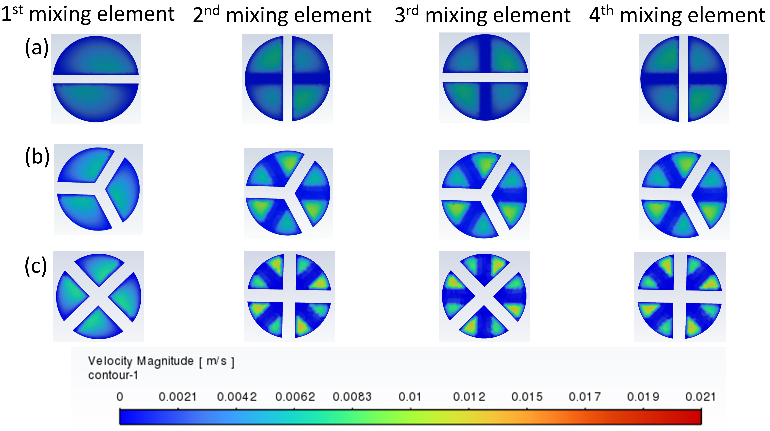
Figure 8 presents the velocity magnitude distribution at different cross-sections along the I-shaped, Y-shaped, and cross-shaped twisted static mixers at Re = 50. The velocity contours show that each mixer geometry generates different internal flow structures.
Figure 8. Velocity magnitude distribution at different cross-sections of the static mixers (Reynolds number (Re) = 50): (a) I-shaped, (b) Y-shaped, and (c) cross-shaped twisted static mixer
In the I-shaped mixer, the velocity distribution is mainly divided by the twisted flat plate. The high-velocity regions around 0.0062 m/s are relatively limited and are mostly formed near the open areas beside the plate. The flow is split into two dominant regions, which results in a simpler velocity pattern. This explains why the concentration redistribution in the I-shaped mixer is less effective than in the modified geometries.
In the Y-shaped mixer, the velocity field becomes more complex due to the three-branch structure. The flow is divided into three main passages, generating more velocity gradients and secondary flow regions. These velocity gradients help stretch and redistribute the tracer, improving the mixing performance compared with the I-shaped mixer.
The cross-shaped mixer produces the most complex velocity distribution. The four-branch geometry creates multiple flow passages and more distributed high-velocity zones around 0.012 m/s across the cross-section. This condition increases flow splitting and radial movement, which are important mechanisms for laminar mixing. The more complex velocity field generated by the cross-shaped element contributes to the better concentration uniformity observed in the concentration contours.
Therefore, the velocity distribution supports the concentration distribution results. The modified Y-shaped and cross-shaped elements generate stronger flow division than the conventional I-shaped element, with the cross-shaped mixer producing the most effective internal flow redistribution.
3.4 Axial concentration distribution
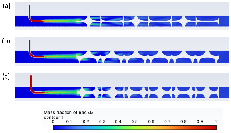
Figure 9 shows the tracer mass fraction distribution along the axial plane of the static mixers at Re = 50. The contours illustrate how the tracer develops from the inlet region and interacts with the twisted elements inside the pipe.
Figure 9. Axial tracer mass fraction distribution of the static mixers (Reynolds number (Re) = 50): (a) I-shaped, (b) Y-shaped, and (c) cross-shaped twisted static mixer
In the I-shaped mixer, the tracer remains relatively concentrated along the central region of the flow for a longer distance. Although the twisted elements split and rotate the flow, the tracer plume remains visible even after several elements. This indicates that the I-shaped geometry provides gradual mixing but requires a longer length to achieve a more homogeneous distribution.
In the Y-shaped mixer, the tracer is more rapidly dispersed after entering the mixer section. The three-branch twisted structure promotes better flow division and increases the contact area between the tracer and the main fluid. As a result, the tracer plume becomes weaker along the downstream direction compared with the I-shaped mixer.
The cross-shaped mixer shows the strongest axial redistribution. The tracer concentration decreases more rapidly along the mixer length because the four-branch structure repeatedly divides and redistributes the flow. This result indicates that the cross-shaped mixer can improve mixing intensity within a shorter axial distance.
The axial concentration contours show that increasing the number of branches in the twisted element improves the mixer's ability to break down the tracer plume and distribute it throughout the pipe.
3.5 Effect of Reynolds number on friction factor
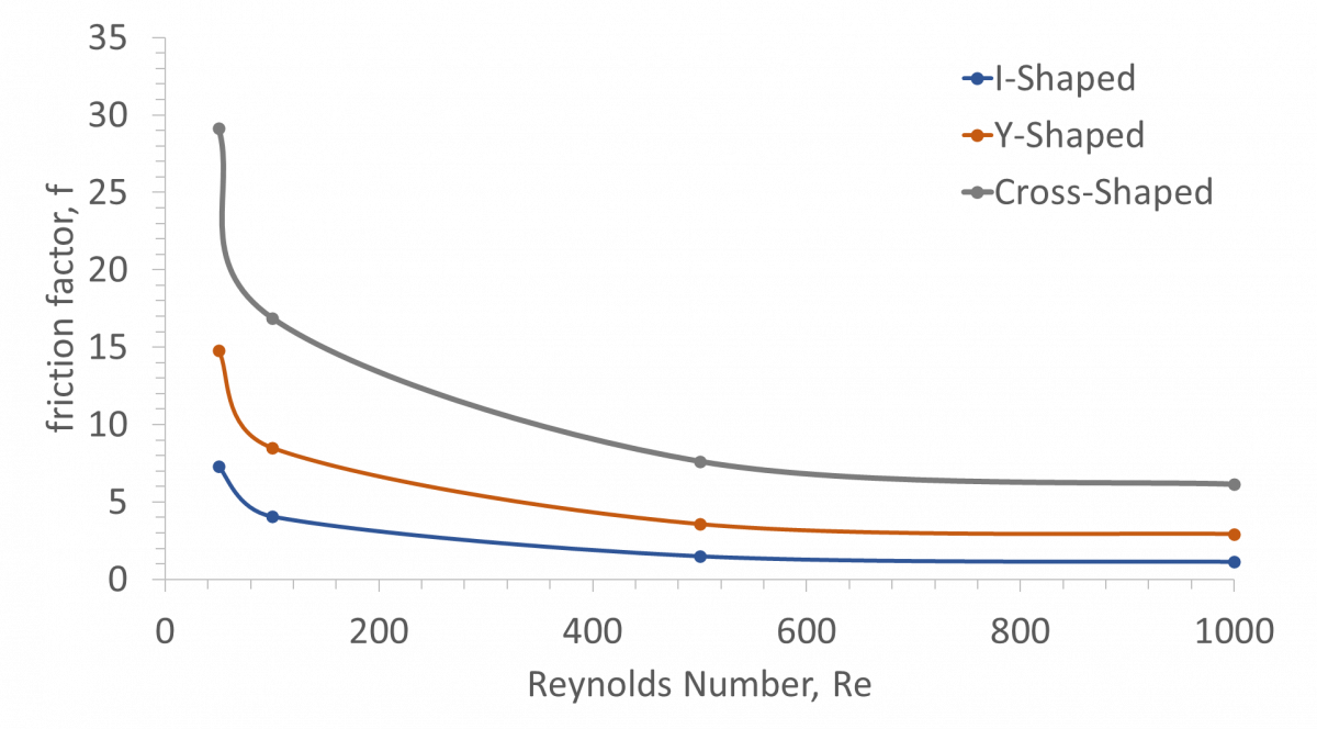
Figure 10 shows the relationship between Re and friction factor for the I-shaped, Y-shaped, and cross-shaped twisted static mixers. For all mixer configurations, the friction factor decreases as the Re increases. This trend is expected in low Re flow because viscous effects dominate. As the Re increases, the relative contribution of viscous resistance decreases, resulting in a lower friction factor.
Figure 10. Effect of Reynolds number (Re) on the friction factor of the I-shaped, Y-shaped, and cross-shaped twisted static mixers
Among the three geometries, the I-shaped mixer produces the lowest friction factor, with a range of 1 to 8. This is because the I-shaped element has the simplest geometry and creates the least obstruction to the flow. The Y-shaped mixer has a higher friction factor, ranging from 2 to 15, than the I-shaped mixer because the three-branch structure increases the wetted surface area and flow blockage. The cross-shaped mixer yields the highest friction factor, ranging from 5 to 30, because its four branches create the greatest flow obstruction.
3.6 Effect of Reynolds number on coefficient of variation
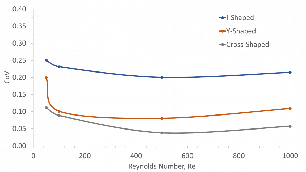
Figure 11 shows the effect of Re on the CoV for the three mixer configurations. The CoV represents the degree of concentration non-uniformity at the outlet. A lower CoV indicates better mixing performance.
Figure 11. Effect of Reynolds number (Re) on coefficient of variation (CoV) of the I-shaped, Y-shaped, and cross-shaped twisted static mixers
The I-shaped mixer shows the highest CoV, ranging from 0.20 to 0.25, over the investigated Re range from 50 to 1000. This indicates that the conventional I-shaped twisted element has the lowest mixing performance among the three configurations. The limited number of flow-splitting paths reduces the mixer's ability to redistribute the tracer effectively across the pipe cross-section.
The Y-shaped mixer produces a lower CoV, ranging from 0.08 to 0.20, than the I-shaped mixer across all Re. This result indicates better mixing performance than the conventional I-shaped design.
The cross-shaped mixer produces the lowest CoV, ranging from 0.04 to 0.11, among all configurations. This shows that the cross-shaped element provides the best mixing uniformity.
For all configurations, the CoV decreases from Re = 50 to approximately Re = 500. This indicates that increasing Re initially strengthens convective redistribution inside the mixer. However, beyond Re = 500, the CoV slightly increases or becomes nearly constant. This behavior may be related to the reduced residence time at higher flow velocity, which limits the available time for diffusion and complete homogenization. Therefore, the best mixing condition appears around Re = 500, where convective deformation and residence time are more balanced.
Although the cross-shaped mixer yields the lowest CoV, this improvement should be interpreted alongside the friction-factor results. The cross-shaped geometry provides the best mixing quality but also produces the highest hydraulic resistance. Therefore, the selection of mixer geometry should consider both mixing uniformity and pressure-drop penalty.
3.7 Engineering comparison and design implication
The comparison between the Y-shaped and cross-shaped mixers should be evaluated from both mixing quality and pumping cost perspectives. The cross-shaped mixer produces the lowest CoV among the investigated configurations, indicating the most uniform outlet concentration distribution. This improvement is caused by its four-branch structure, which enhances flow splitting, radial redistribution, and scalar stretching. Therefore, the cross-shaped mixer is preferable when the main design target is maximum mixing uniformity, especially in compact systems where the available mixing length is limited or in processes where concentration uniformity is more critical than energy consumption.
However, the cross-shaped mixer also produces the highest friction factor. The additional branches increase the blockage ratio, the wetted surface area, the local velocity gradients, and the viscous dissipation. As a result, the pressure-drop penalty and the required pumping power increase. Therefore, the cross-shaped configuration is more suitable for applications where sufficient pump capacity is available, and the additional hydraulic resistance can be tolerated.
In contrast, the Y-shaped mixer provides an intermediate performance. Its three-branch structure improves flow splitting and radial transport compared with the conventional I-shaped mixer, but its hydraulic resistance remains lower than that of the cross-shaped mixer. Thus, the Y-shaped mixer is preferable when a compromise between improved mixing and moderate pressure drop is required. This configuration is more appropriate for systems with pumping-power limitations, pressure-drop constraints, or continuous operation where energy efficiency is an important consideration.
Therefore, the cross-shaped mixer should be selected for high-uniformity mixing applications, while the Y-shaped mixer is more suitable for energy-conscious applications requiring acceptable mixing enhancement with lower hydraulic penalty. The optimum configuration should be chosen based on the allowable pressure drop, available pumping capacity, required outlet CoV, and process-specific mixing requirements.
A three-dimensional CFD simulation was conducted to investigate the effect of element cross-sectional shape on the mixing performance of twisted static mixers at low Re. Three mixer configurations were compared, namely the conventional I-shaped, the Y-shaped, and the cross-shaped twisted static mixer. The performance of each mixer was evaluated using the CoV and the friction factor.
The results show that the cross-sectional shape of the twisted element significantly influences the flow structure and mixing performance. The I-shaped mixer produces the simplest flow pattern and the lowest friction factor, but it gives the highest CoV. This indicates that the conventional I-shaped twisted element has limited capability to redistribute the tracer uniformly across the pipe section.
The Y-shaped mixer improves the mixing performance compared with the I-shaped mixer. The three-branch twisted geometry increases flow splitting and radial redistribution, resulting in lower CoV values. However, this improvement is accompanied by a higher friction factor due to the increased obstruction inside the pipe.
The cross-shaped mixer provides the best mixing performance among the three configurations. The four-branch twisted element generates more flow paths, stronger tracer stretching, and better radial redistribution, resulting in the lowest CoV across the investigated range of Re. However, the cross-shaped mixer also results in the highest friction factor due to its greater blockage and more complex internal geometry.
Overall, the cross-shaped twisted static mixer is the most effective configuration when the main objective is maximum mixing uniformity. Meanwhile, the Y-shaped twisted static mixer can be considered a promising alternative when both mixing performance and hydraulic resistance are taken into account. These results confirm that modifying the cross-sectional shape of twisted static mixer elements can be an effective approach for improving laminar mixing performance. Therefore, the optimum static mixer geometry depends on the required outlet uniformity, allowable pressure drop, available pump capacity, and process-specific requirements.
This study is limited to a CFD-only approach under idealized assumptions, including steady laminar flow and identical water/brine properties. Therefore, the reported CoV and friction-factor values should be interpreted as comparative numerical indicators.
|
V |
velocity, m/s |
|
Y |
mass fraction |
|
D |
molecular diffusion coefficient, m2/s |
|
Greek symbols |
|
|
ρ |
density, kg/m3 |
|
µ |
dynamic viscosity, kg/(m‧s) |
|
Subscripts |
|
|
A |
tracer |
|
AB |
tracer and water |
[1] Yu, Y.F., Yu, S.Y., Meng, H.B., Xia, R.Y., Wang, D.D., Han, Z.Y. (2026). Investigation of mass transfer characteristics in CO2 absorption within high-efficiency carbon capture static mixer based on CFD and experimental methods. Chemical Engineering Journal, 530: 173271. https://doi.org/10.1016/j.cej.2026.173271
[2] Gao, Y., Lu, B., Zhang, X.X., et al. (2026). Design and optimization of a bionic starfish-inspired inlet configuration static mixer using response surface methodology for efficient natural gas-hydrogen mixing. Chemical Engineering and Processing-Process Intensification, 223: 110775. https://doi.org/10.1016/j.cep.2026.110775
[3] Lei, H., Guan, X.H., Sun, Y.K., Yan, H.X. (2022). A novel design of in-line static mixer for permanganate/bisulfite process: Numerical simulations and pilot-scale testing. Water Environment Research, 94(5): e10725. https://doi.org/10.1002/wer.10725
[4] Huang, Y., Hao, M.Q., Yu, S.Y., Huang, H., Liu, G. (2026). A modified static mixer proposed for efficient blending of hydrogen and methane. International Journal of Hydrogen Energy, 222: 154254. https://doi.org/10.1016/j.ijhydene.2026.154254
[5] Albertazzi, J., Busini, V., Rota, R. (2024). Comparison through a CFD approach of static mixers in an emulsification process. International Journal of Thermofluids, 22: 100708. https://doi.org/10.1016/j.ijft.2024.100708
[6] Ghanem, A., Lemenand, T., Della Valle, D., Peerhossaini, H. (2014). Static mixers: Mechanisms, applications, and characterization methods-A review. Chemical Engineering Research and Design, 92(2): 205-228. https://doi.org/10.1016/j.cherd.2013.07.013
[7] Shao, W.Y., Pan, X.S., Zhao, Z.R., Cui, S.M. (2021). Effects of process parameters on the size of low-molecular-weight chitosan nanoparticles synthesized in static mixers. Particulate Science and Technology, 39(8): 911-916. https://doi.org/10.1080/02726351.2020.1859027
[8] Meijer, H.E.H., Singh, M.K., Anderson, P.D. (2012). On the performance of static mixers: A quantitative comparison. Progress in Polymer Science, 37(10): 1333-1349. https://doi.org/10.1016/j.progpolymsci.2011.12.004
[9] Von Damnitz, L., Anders, D. (2025). A review on the mixing quality of static mixers. ChemEngineering, 9(6): 128. https://doi.org/10.3390/chemengineering9060128
[10] Valdés, J.P., Kahouadji, L., Matar, O.K. (2022). Current advances in liquid-liquid mixing in static mixers: A review. Chemical Engineering Research and Design, 177: 694-731. https://doi.org/10.1016/j.cherd.2021.11.016
[11] Bennour, E., Kezrane, C., Kaid, N., Alqahtani, S., Alshehery, S., Menni, Y. (2023). Improving mixing efficiency in laminar-flow static mixers with baffle inserts and vortex generators: A three-dimensional numerical investigation using corrugated tubes. Chemical Engineering and Processing-Process Intensification, 193: 109530. https://doi.org/10.1016/j.cep.2023.109530
[12] Jiang, X.R., Yang, N., Wang, R.J. (2021). Effect of aspect ratio on the mixing performance in the Kenics static mixer. Processes, 9(3): 464. https://doi.org/10.3390/pr9030464
[13] Pezo, M., Pezo, L., Lončar, B., Kojić, P., Jovanović, A.A. (2025). A comprehensive review of discrete element method studies of granular flow in static mixers. Processes, 13(11): 3522. https://doi.org/10.3390/pr13113522
[14] Abou-Hweij, W., Azizi, F. (2025). Hydrodynamic and mixing characterization of a novel static mixer geometry: A numerical study. Chemical Engineering Communications, 212(11): 1621-1640. https://doi.org/10.1080/00986445.2025.2484750
[15] Nyande, B.W., Mathew Thomas, K., Lakerveld, R. (2021). CFD analysis of a Kenics static mixer with a low pressure drop under laminar flow conditions. Industrial & Engineering Chemistry Research, 60(14): 5264-5277. https://doi.org/10.1021/acs.iecr.1c00135
[16] Jiang, X.R., Xiao, Z.D., Jiang, J.N., Yang, X.X., Wang, R.J. (2021). Effect of element thickness on the pressure drop in the Kenics static mixer. Chemical Engineering Journal, 424: 130399. https://doi.org/10.1016/j.cej.2021.130399
[17] Qiao, Y., Zheng, L.Y., Guo, K., et al. (2024). Numerical study of flow field and mixing performance of a new curved-sheet blade-folded static mixer. Industrial & Engineering Chemistry Research, 63(17): 7836-7852. https://doi.org/10.1021/acs.iecr.3c04601
[18] Menni, Y., Sari Hassoun, Z., Kaid, N., Alqahtani, A.A., Alqahtani, S., Jazaa, Y. (2025). Numerical analysis of blade height ratio effects on mixing efficiency and energy consumption in triple-blade concentric double-helix static mixers. Physics of Fluids, 37(2): 023602. https://doi.org/10.1063/5.0245378
[19] Regner, M., Östergren, K., Trägårdh, C. (2006). Effects of geometry and flow rate on secondary flow and the mixing process in static mixers-a numerical study. Chemical Engineering Science, 61(18): 6133-6141. https://doi.org/10.1016/j.ces.2006.05.044
[20] Mahammedi, A., Ameur, H., Ariss, A. (2017). Numerical investigation of the performance of Kenics static mixers for the agitation of shear thinning fluids. Journal of Applied Fluid Mechanics, 10(3): 989-999. https://doi.org/10.18869/acadpub.jafm.73.240.27314
[21] Šir, J., Lecjaks, Z. (1982). Pressure drop and homogenization efficiency of a motionless mixer. Chemical Engineering Communications, 16(1-6): 325-334. https://doi.org/10.1080/00986448208911104
[22] Al-Atabi, M. (2011). Design and assessment of a novel static mixer. The Canadian Journal of Chemical Engineering, 89(3): 550-554. https://doi.org/10.1002/cjce.20412