Maarouf Ahmad | Ali A. Battawi* | Balsam H. Abed
© 2026 The authors. This article is published by IIETA and is licensed under the CC BY 4.0 license (http://creativecommons.org/licenses/by/4.0/).
OPEN ACCESS
External environmental conditions significantly influence the operational efficiency and economic performance of marine power plants. Understanding the magnitude of this influence is essential for improving the reliability and efficiency of marine propulsion systems. In this study, the influence of environmental factors on the performance of marine diesel engine charging systems is investigated using a mathematical modeling approach. A comprehensive mathematical model representing the interaction between the external environment, the ship propulsion complex, the main engine, and the charging system was developed. The mathematical model was transformed using modern computer applications and software into a computer program that simulates the operation of marine power stations and the effect of external environmental factors on their performance. To validate the developed model, a set of experimental studies was conducted on marine propulsion stations installed on ships operating in the Eastern Mediterranean region. The obtained results confirmed the accuracy of the developed model and demonstrated its ability to predict propulsion performance under varying environmental conditions. Based on the conducted analysis, a methodology for selecting optimal operating modes of marine propulsion stations under changing environmental parameters was developed. Additionally, several practical recommendations aimed at improving the operational efficiency of marine propulsion systems were proposed.
marine diesel engines, environmental factors, turbocharging systems, ship propulsion performance, fuel consumption, navigation range, mathematical modeling
Marine diesel propulsion stations represent the most widely used propulsion systems in modern maritime transport. Their operational efficiency directly influences ship performance, fuel consumption, and operating costs. Environmental conditions such as atmospheric temperature, pressure, humidity, sea state, and wind characteristics significantly affect the operational parameters of marine engines and propulsion systems.
Determining the influence of these environmental parameters through full-scale experimental studies requires considerable financial and technical resources, including fuel consumption, lubrication oil usage, and reduction of engine lifetime. Therefore, mathematical modeling methods are widely used for analyzing the interaction between propulsion systems and external environmental conditions.
In this research, the performance of the integrated system consisting of the external environment – marine propulsion complex – main engine – charging system is investigated using a comprehensive mathematical modeling approach [1, 2].
The main objectives of this research are [3]:
Developing scientific methods for determining the characteristics of air-charging systems in marine diesel engines.
Modeling environmental variations in the Eastern Mediterranean Sea.
Investigating the combined influence of environmental factors on the operational efficiency of marine diesel propulsion stations installed on Syrian surface ships.
Identifying the main directions for improving the performance efficiency of a marine propulsion station operating in the regional maritime environment.
The issues raised in this research were addressed in two ways:
1. Mathematical modeling;
2. Verification of the results of mathematical modeling through practical experiments.
3.1 Mathematical model of the marine propulsion station
The mathematical model of the marine propulsion station developed in this research can solve the following problems:
1. Determining the maximum and minimum speeds of the vessel under varying external environmental parameters or operating conditions;
2. Determining the hourly fuel consumption of the main engines and the entire propulsion station at any vessel speed;
3. Determining the cost per hour of cruising from the propulsion station's operating expenses at any vessel speed;
4. Determining the vessel's cruising range at any vessel speed.
3.2 Preparing the initial data matrix
The mathematical model of the external environment of the Eastern Mediterranean region and the performance of the shipborne power plants enable the implementation of various tests for the "External Environment - Offshore Propulsion Complex" system. To obtain a stable mathematical prediction of the values of the indicators (parameters) of the effectiveness of the shipborne propulsion complex, the number of tests to be conducted must be determined. It is suggested that the number of tests should fall within a certain range [4], while another criterion is proposed for determining the number of tests through the stability of the mathematical prediction in the form of the relationship [5]:
$U=\frac{1}{M_1(Z)}\left[M_1(Z)-M_2(Z)\right]$ (1)
where, $M_1(Z)$ and $M_2(Z)$ are the mathematical predictions of the Z function corresponding to two equal sizes of statistical trial matrices, each of which is determined by the relation:
$M(Z)=\frac{1}{N} \sum_{n=1}^N Z_n$ (2)
The stability of the mathematical prediction $(U \approx 0)$ occurs rapidly, and in the marine power station problems addressed in this research, stability occurs at $(N=70 / 150)$. In the experiments of this research, the number was adopted $(N=100)$. For each ship model, independently and at a specific step, the possible speed spectrum from $v_{\text {min}}$ to $v_{\text {max}}$ is assumed, and then the mathematical prediction and dispersion (squared deviation) are calculated for the values of three parameters: hourly fuel consumption $B$, cost per hour of sailing $C_{\text {rhe}}$, and sailing range $\left(S_v\right)$. For fast ships, three sets of statistical data were obtained, two of which were for individual propeller working cases (Table 1).
Table 1. Studied speed ranges and operating conditions of the main propulsion station on high-speed vessels
|
Operating Conditions of the Propulsion Station |
Studied Speed Ranges of the Boat [Kn] |
|
Operation of three fixed-pitch propellers $z_p=3$ |
10.5/40 |
|
Operation of two fixed-pitch propellers $z_p=2$ |
8.4/29.4 |
|
Operation of one fixed-pitch propellers $z_p=1$ |
8.4/25.4 |
Statistical data were obtained, two of which were for individual propeller working cases (Table 1).
For ship voyages ($k_N$) and time elapsed after berthing ($T_{\text {exp}}$) during two different climatic seasons, both regression and correlational (reciprocal) analysis were used. For example, for high-speed vessels operating in independent propulsion groups, the regression relationships for hourly fuel consumption at the power station $(B[k g / h])$, ship voyage range $\left(S_v[\right.$mile$\left.]\right)$, and hourly voyage cost $\left(C_{\text {rhe}}[u . e / h]\right)$ are as follows:
${January}(S-1) B=2491.1 \cdot \bar{v}_i-94.62 \cdot K_N+44.11 \cdot T_{{exp}}$ (3)
${August}(S-2) B=2500 \cdot \bar{v}_i-121.4 \cdot K_N+34.6 \cdot T_{\exp}$ (4)
${January}(S-1) S_v=1765.4-60.97 \cdot T N \bar{v}_{i_{{exp}}}$ (5)
August $(S-2) S_v=2151-57.6 \cdot T N \bar{v}_{i_{{exp}}}$ (6)
${January}(S-1) C_{r h e}=597.9 \cdot \bar{v}_i-22.74 \cdot K_N+10.59 \cdot T_{e x p}$ (7)
${August}(S-2) C_{r h e}=600 \cdot \bar{v}_i-29.15 \cdot K_N+8.3 \cdot T_{e x p}$ (8)
To assess the quality of the choice of return relations (functions), the correlation constant is used, which expresses the strength of the linear relationship of the variable $y_i\left(B, C_{\text {rhe}}, S_v\right)$ to the set of variables $X_i\left(v_i, T N_{\text {exp}}\right)$, according to the relationship:
$R=\sqrt{1-\left(\sum e_i^2 / \sum\left(Y_i-\bar{Y}\right)^2\right)}$ (9)
where, $\sum e_i^2$ - the sum of the squares of the actual deviations of the values (of the observations) from the return curve; $\sum\left(Y_i-\bar{Y}\right)^2$ - the sum of the squares of the actual deviations of the values (of the observations) from the mathematical expectation.
In this research, calculations were performed using the software package as follows: for a range of diverse marine propulsion systems; for all use cases of each system studied; for all parameter ($B, S_v, C_{r h e}$) return relationships, within $95 \%$ certainty ranges, within which the expected value of each parameter $\left(B, S_v, C_{r h e}\right)$ can be guaranteed. Based on initial statistical data and using the Math Cad software package to determine the values of: hourly fuel consumption, vessel cruising range, and hourly cruising cost according to nonlinear return relationships, the relationships (3/8) were transformed into the following form:
January $(S-1) B=-533+2726 \cdot \bar{v}_i-242 \cdot \bar{v}_i^2-92 \cdot K_N+44 \cdot T_{{exp}}$ (10)
August $(S-2) B=-624+2460 \cdot \bar{v}_i+44 \cdot \bar{v}_i^2-122 \cdot K_N+35 \cdot T_{{exp}}$ (11)
January $(S-1) S_v=2315-3860 \cdot \bar{v}_i+2616 \cdot \bar{v}_i^2+187 \cdot K_N-58 \cdot T_{\exp}$ (12)
August $(S-2) S_v=2430-4140 \cdot \bar{v}_i+2470 \cdot \bar{v}_i^2+283 \cdot K_N-56 \cdot T_{{exp}}$ (13)
January $(S-1) C_{r h e}=-127.9+654.2 \cdot \bar{v}_i-58.2 \cdot \bar{v}_i^2-22.1 \cdot K_N+10.53 \cdot T_{{exp}}$ (14)
August $(S-2) C_{r h e}=-149.7+589 \cdot \bar{v}_i+10.5 \cdot \bar{v}_i^2-29.2 \cdot K_N+8.31 \cdot T_{{exp}}$ (15)
A mathematical model representing the operational behavior of a marine propulsion station was developed. The model enables the determination of several operational parameters, including [6]:
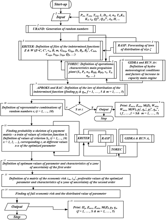
Figure 1 illustrates the overall structure of the mathematical model that represents the performance (work) of a marine propulsion station.
Figure 1. General diagram of the mathematical representational model for the operation of a marine propulsion station (algorithm)
The model was developed based on operational data collected from ships operating in the Eastern Mediterranean region. This mathematical model allows for the identification of two types of specifications [4]:
I. First Type: A set of indicators that allows comparison between the specifications of the ship propulsion station, such as: the maximum speed $\left(v_{\max}\right)$ and minimum speed $\left(v_{\min}\right)$ of the ship, total fuel consumption $(B)$, the required power from the main propulsion station $\left(P_{e \Sigma}\right)$, and electrical loads $\left(P_{e D G}\right), \ldots$, etc.
II. Second Type: A set of indicators that can be used as criteria to evaluate the performance efficiency of the ship propulsion station, such as: the cost per hour of navigation, the amount of metal constituting the propulsion station $\left(\gamma_{S P P}\right)$ and the ship as a whole $\left(\gamma_{\text {Ship}}\right)$, fuel consumption per nautical mile traveled by the ship $\left(b_{\text {mile}}\right)$, hourly fuel consumption $\left(b_h\right)$, the annual investment $\operatorname{cost}\left(C_y\right)$, and the total cost over the entire service life $\left(C_{\Sigma}\right)$.
Marine propulsion stations are characterized by thermodynamic indicators, power indicators, mass indicators, cost indicators, and others. The random numbers required to determine the inverse integrals of the distribution functions of external variables are obtained using the standard instruction (subroutine) URAND, block (2).
The subroutine KRITER, block (3), is considered central, and its main function is to determine the performance (efficiency) criteria of the ship power plant, as well as the criteria for its comparison with other possible configurations (cases) of power plants.
In general, by means of block 3 (KRITER), matrices of parameter values describing the various operational characteristics of the marine propulsion station are obtained. These matrices represent a set of statistical values generated by the computer and describe different characteristics of the ship and its onboard power plant, such as: absolute costs $(C)$ and relative costs $\left(C^{\prime}\right)$, average economic speed $\left(v_s\right)$, fuel consumption $(B)$, ship hull mass $\left(G_{\text {ship}}\right)$, and propulsion station mass $\left(G_{\text {SPP}}\right)$, onboard fuel reserve $\left(Q_{f i}\right)$, ship displacement $\left(D_i\right)$, costs allocated for intermediate overhaul ($B_p$), other types of maintenance and repair costs ($\mathrm{B}^{\prime} p$), service costs over a specified standard period or over the entire investment (service) cycle $\left(T_{\text {cycle}}\right)$, ship construction costs $\left(C_b\right)$, positioning costs ($C_{\text {base}}$) costs of routine repairs and inspections ($C_r$), costs of replacing certain equipment ($C_{r p}$), fuel cost $\left(C_f\right)$, oil cost $\left(C_{\text {oil}}\right)$, crew expenses $\left(C_{\text {pers}}\right)$, and other total investment costs $\left(C_{\Sigma}\right)$, fuel consumption per hour $\left(b_h\right)$ and per mile $\left(b_{\text {mile}}\right)$, the amount of metal constituting the propulsion station $\left(\gamma_{\text {SPP}}\right)$, Total Investment Costs $\left(C_{\text {exp}}^a\right)$ and average annual costs $\left(C_y\right)$.
The criteria (C) and (C') are calculated and determined for all propulsion station configurations for each of the studied ships over the entire investment spectrum. The optimal propulsion station configurations are those characterized by minimum values of the parameters (C) and (C').
A set of calculations is performed in block 3 with the assistance of the subroutine RASP (block 4) and the subroutine TOREC (block 5). The latter subroutine TOREC, in turn, interacts with the subroutine GIDRA and the subroutine RUN Av (block 6).
The subroutine TOREC is dedicated to determining (calculating) the operational (investment) characteristics of the ship propulsion station installed on board the vessel. The hourly fuel consumption is calculated independently (separately) for each of the Main Engines $\left(B_{M E}\right)$, the diesel engines used for electrical power generation (Diesel Generator) $\left(B_{D G}\right)$, and auxiliary steam generators, if present (auxiliary steam generator) $\left(B_{A S G}\right)$, on a monthly and yearly basis. These values are then aggregated while considering the duration of navigation periods and the number of operating main and auxiliary engines required to ensure the assumed ship speed.
To determine the influence of environmental factors (external conditions), the subroutine TOREC refers (returns) to the subroutines GIDRA and RUN Av. During this process, the subroutine GIDRA determines the hydrometeorological parameters, while the subroutine RUN Av calculates the values of the power correction coefficients $A_v$, which are considered random variables that allow, with good accuracy, the determination of the expected ship speed, the load level of the main and auxiliary engines and auxiliary boilers, as well as the necessity and method of applying individual operating modes for the main engines.
The subroutine RUN analyzes the changes in the propulsion system characteristics and selects the appropriate operating modes for the ship power plant.
According to hydrometeorological conditions, the voyage route (L) is divided into four segments of different lengths (L1), (L2), (L3), (L4). During this process, the economic speed of the ship is calculated for each segment while taking into account the spectrum of operating modes.
The list of calculated specifications includes:
Using the subroutine GIDRA, one of the possible configurations of hydrometeorological factors prevailing in the Eastern Mediterranean region has been determined, consisting of:
3.3 Environmental parameters modeling
The model incorporates a set of environmental variables representing hydrometeorological conditions, including [7, 8]:
These parameters were modeled using statistical distributions derived from real environmental data recorded in the Eastern Mediterranean maritime region [9].
The mathematical model of the external environment of the Eastern Mediterranean region and the performance of the shipborne propulsion station enable the implementation of various tests for the "external environment-marine propulsion system." To obtain a stable mathematical prediction of the values (parameters) of the effectiveness of the shipborne propulsion system investment, the number of tests to be conducted must be determined. It is suggested that the number of tests should fall within the range of (50/100) [10], while another criterion is proposed for determining the number of tests based on the stability of the mathematical prediction [11].
For each vessel type, independently and at a specific step, the possible speed spectrum from $v_{\min}$ to $v_{\max}$ is assumed. Then, the mathematical prediction and dispersion (squared deviation) are calculated for the values of three parameters: hourly fuel consumption (B), cost per hour of sailing ($C_{{rhe}}$), and cruising range ($S_v$). For high-speed vessels, three sets of statistical data were obtained, two of which were for individual propeller operating conditions, as shown in Table 1 [12].
Statistical data were obtained during simulated experiments on the "external environment - marine propulsion system" on fast vessels using a computer program presented in tabular form. This data was collected to study the impact of climatic conditions and operational factors on the performance of the propulsion system. Table 2 includes some of this data for fast vessels operating with only two propellers $\left(z_p=2\right)$.
Table 2. Some statistical data obtained from experiments conducted on the mathematical model “External Medium – Marine Propulsion station” for high-speed vessels at (zₚ = 2)
|
Season |
Texp (month) (Elapsed Time After Docking) |
Sailing Intensity Constant kN |
Successful Experiments |
Relative Ship Speed v̄ᵢ |
Fuel Consumption B (kg/h) (Mean / Standard Deviation) |
Cost per Hour Crhe (u.e) (Mean) |
Sailing Range Sv (mile) (Mean Standard Deviation) |
|
1 |
0 |
0 |
100 |
0.20 |
361.539 |
86.822 |
840.375 |
|
1267.179 |
72.990 |
5447.661 |
|||||
|
35.597 |
8.543 |
73.808 |
|||||
|
1 |
0 |
0.020 |
100 |
0.550 |
805.588 |
193.394 |
1076.544 |
|
2390.034 |
137.666 |
4078.715 |
|||||
|
48.888 |
11.733 |
63.865 |
|||||
|
1 |
3 |
0 |
100 |
0.450 |
730.240 |
175.310 |
970.217 |
|
3213.242 |
185.081 |
5173.95 |
|||||
|
56.685 |
13.604 |
71.930 |
|||||
|
1 |
3 |
0.020 |
100 |
0.400 |
593.945 |
142.599 |
1047.882 |
|
970.332 |
55.890 |
2665.046 |
|||||
|
31.150 |
7.476 |
51.624 |
|||||
|
1 |
6 |
0.020 |
100 |
0.300 |
579.374 |
139.102 |
1047.882 |
|
3161.892 |
182.125 |
2665.046 |
|||||
|
56.231 |
13.495 |
51.624 |
3.4 Simulation procedure
The developed mathematical model was implemented using computational tools including [13, 14]:
Simulink/MATLAB
Microsoft Excel
Mathcad
The simulation model integrates several computational subroutines responsible for evaluating propulsion performance, generating environmental parameters, and determining operational performance indicators [15].
3.5 Experimental validation
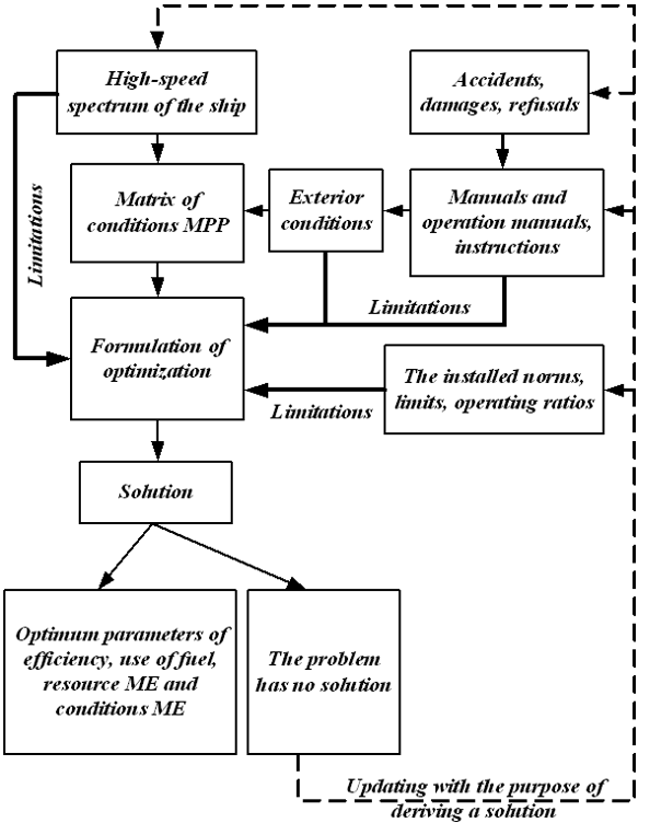
The selection and rationale for the operation of diesel propulsion station used on ships begins with formulating a system matrix that considers the expected sailing conditions and the anticipated technical condition of the ship and all its components. Initially, the following preliminary data are assumed: sailing speed or speed range; external environmental factors (climatic and operational factors); and constraints (precautions, standards, efficiency constants, service life, etc.).
When determining (assuming) the required speed spectrum, the formation of the work systems matrix and the solution of the example problem are done according to the algorithm shown in Figure 2, Case No. 1.
Figure 2. Algorithm for forming a matrix of working systems to solve the example problem (Case No. 1)
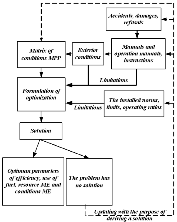
Figure 3. Algorithm for forming a matrix of working systems to solve the example problem (Case No. 2)
When a specific range of required speeds exists, the problem is solved according to the sequence shown in Figure 3, Case No. 2 [16, 17].
To verify the accuracy of the developed model, a series of experimental studies were conducted on a marine propulsion station installed on operational ships [18].
Statistical experiments were carried out to analyze the interaction between environmental conditions and propulsion system performance. The results obtained were processed using regression and correlation analysis methods to determine the relationships between ship speed, fuel consumption, navigation cost, and navigation range.
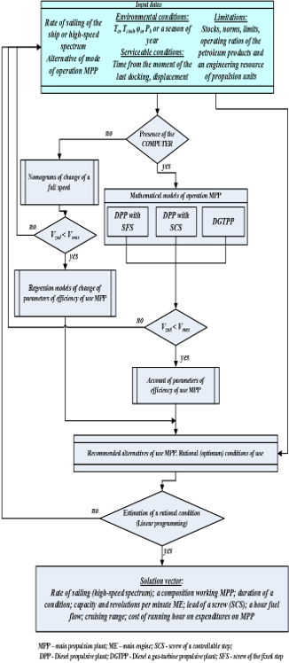
The diagram of the method used to justify the systems suitable for the use of main power stations on ships is shown in Figure 4.
Figure 4. Diagram of the method used to justify and select suitable systems for use in main power stations on ships
Tables 3 and 4 illustrate some of the results of the experiments carried out on this mathematical model, and compare them with the results obtained through conducting some practical experiments on ships during their investment in the Eastern Mediterranean region (under equivalent initial conditions), which confirmed the accuracy of the results of this model and the possibility of using it in research and studies related to the design and investment of marine power stations.
Results obtained from the mathematical model were compared with operational data collected from marine engines operating under real maritime conditions [14, 19].
The comparison demonstrated a high level of agreement between simulated and experimental results for parameters such as engine rotational speed, Engine power output, and hourly fuel consumption.
The analysis also revealed that the most significant factors affecting marine propulsion performance include: Hull fouling, Sea state conditions, Variations in external air temperature, and individual propeller operating modes [19].
Based on the calculations, a set of recommendations, guidelines, and practical suggestions can be formulated to ensure increased efficiency in the use of marine propulsion stations on ships in the Eastern Mediterranean region. The most important of these are:
1. During the daily operation of surface vessels, the impact of external environmental factors on their technical specifications and the performance indicators of the onboard diesel and hybrid propulsion station must be considered.
Table 3. Performance of all propulsion sets
|
Ship Speed |
Engine Speed M504, min-1 |
Power Produced by One Engine M504, kW |
Hourly Fuel Consumption in Power Plant, kg/h |
|||
|
|
Actual Data (Operational Records) |
Mathematical Model Results |
Actual Data (Operational Records) |
Mathematical Model Results |
Actual Data (Operational Records) |
Mathematical Model Results |
|
14 |
800 |
814 |
404 |
405 |
268 |
280 |
|
16 |
1000 |
1072 |
713 |
739 |
501 |
491 |
|
21 |
1200 |
1274 |
1102 |
1110 |
785 |
731 |
|
29 |
1500 |
1514 |
1911 |
1907 |
1266 |
1258 |
|
30 |
1550 |
1542 |
2058 |
1995 |
1330 |
1318 |
|
35 |
1700 |
1724 |
2572 |
2561 |
1709 |
1739 |
|
37 |
1800 |
1848 |
2866 |
2890 |
1957 |
2091 |
Table 4. Performance with two propulsion sets (Third Set Stopped)
|
Ship Speed |
Engine Speed M504, min-1 |
Power Produced by One Engine |
Hourly Fuel Consumption in Power Plant |
|||
|
Actual Data |
Model Results |
Actual Data |
Model Results |
Actual Data |
Model Results |
|
|
12 |
800 |
1000 |
389 |
401 |
204 |
212 |
|
18 |
1200 |
1190 |
1470 |
1312 |
616 |
626 |
|
25 |
1500 |
1524 |
2330 |
2349 |
1080 |
1164 |
2. The use of modern ship-docking methods to clean hulls and propellers of fouling, and the application of modern anti-fouling paints, plays a significant role in maintaining the required speed of the vessel (for an extended period after dry-docking), thus ensuring a long cruising range with fuel economy.
3. To maintain the required level of technical readiness of vessels, periodic inspections and planned repairs must be carried out on schedule. Emphasis should also be placed on cleaning compressor inlets of deposits and salts, adjusting and calibrating gas and fuel distribution mechanisms in diesel and gas turbine engines, and maintaining the high technical condition of control and automation equipment, monitoring, alarm, and protection systems.
4. Qualifying and training ship crews to enable them to assess the consequences and results of the impact of external environmental and operational factors on the performance of offshore power plants, as well as to detect changes occurring during this time, and to take all appropriate and correct measures to ensure the ship can fulfill its assigned tasks.
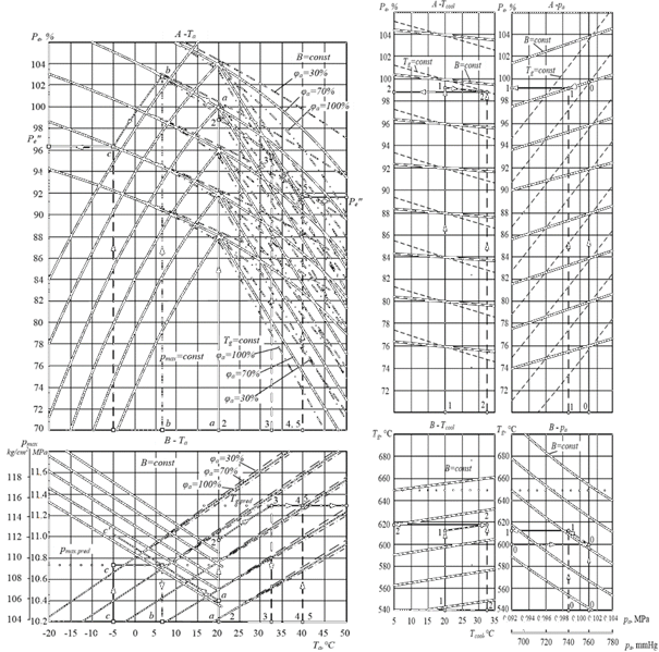
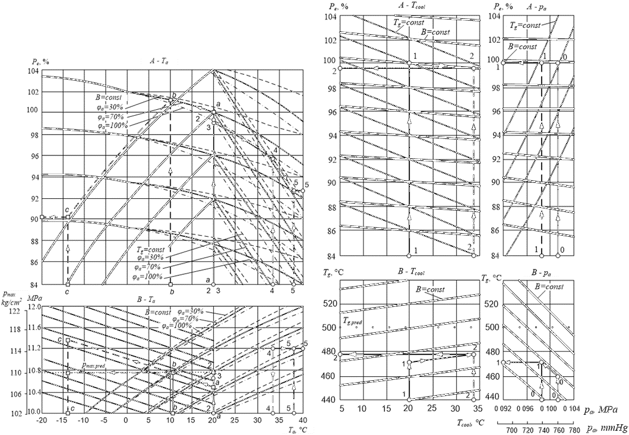
5. Using the computer program for the mathematical model developed in this research, a set of nomograms was generated for some specific operational scenarios. Figures 5 and 6 illustrate two examples of these nomograms, which are used to determine the values of power changes as a function of changes in atmospheric pressure, cooling water temperature, and ambient air temperature and humidity, at a constant fuel quantity or exhaust gas temperature at the turbine inlet, and at low temperatures at a constant maximum combustion pressure.
Figure 5. Diagrams (nomograms) to determine the effect of changes in the external environment on the specifications (characteristics) of four-stroke marine engines used on ships
Figure 6. Diagrams (nomograms) to determine the effect of changes in the external environment on the specifications (characteristics) of two-stroke marine engines used on ships
Their parameters such as cooling water temperature, air humidity, and ship displacement were found to have a comparatively smaller influence on propulsion performance.
The research resulted in the following main conclusions:
The developed model can be used as an effective tool for analyzing and optimizing marine propulsion systems during both design and operational stages.
Future research may focus on extending the developed mathematical model to include hybrid marine propulsion systems and alternative fuels. In addition, integrating real-time environmental monitoring systems with propulsion control algorithms could further enhance the operational efficiency of marine vessels.
[1] Acciaro, M. (2026). Future maritime trade flows and climate change. In Marine Propulsion for Decarbonization, Elsevier, pp. 5-38. https://doi.org/10.1016/C2023-0-01368-1
[2] Kirketerp-Møller, T., Hyldgaard, M.W., Cai, J., Dodis, A.I., Rytter, N.G.M. (2025). Data-driven predictive maintenance for two-stroke marine diesel engines using machine learning and MLOps. Journal of Ocean Engineering and Science, 11(1): 278-296. https://doi.org/10.1016/j.joes.2025.11.011
[3] Luo, Y., Kong, L., Fang, S., et al. (2024). Reviews on the power management for shipboard energy storage systems. Sustainable Horizons, 9: 100094. https://doi.org/10.1016/j.horiz.2024.100094
[4] Chen, Z., Shi, F., Li, J., Li, G. (2026). Simulation of a four-stroke diesel engine for propulsion in wave. Algorithms, 19(5): 421. https://doi.org/10.3390/a19050421
[5] Sakellaridis, N.F., Raptotasios, S.I., Antonopoulos, A.K., Mavropoulos, G.C., Hountalas, D.T. (2015). Development and validation of a new turbocharger simulation methodology for marine two stroke diesel engine modelling and diagnostic applications. Energy, 91: 952-966. https://doi.org/10.1016/j.energy.2015.08.049
[6] Geng, P., Hu, X., Lin, X. (2025). Effects of oxygen enrichment and air humidification on the combustion and emissions of the biodiesel marine diesel engine. Journal of Marine Science and Engineering, 13(2): 271. https://doi.org/10.3390/jmse13020271
[7] Mizythras, P., Boulougouris, E., Theotokatos, G. (2022). A novel objective oriented methodology for marine engine–turbocharger matching. International Journal of Engine Research, 23(12): 2105-2127. https://doi.org/10.1177/14680874211039705
[8] Yu, H., Gao, J., Zhang, P., et al. (2024). The impact of scavenging air state on the combustion and emission performance of marine two-stroke dual-fuel engine. Scientific Reports, 14(1): 15776. https://doi.org/10.1038/s41598-024-66826-z
[9] Spyrou, K.J., Themelis, N. (2025). Innovations in Sustainable Maritime Technology—IMAM 2025: Ship Motions, Hydrodynamics, Propulsion. Springer Nature.
[10] Atak, Ü. (2026). GaussianCopula-based synthetic data generation for turbocharger fault scenario simulation and SFOC degradation modelling in two-stroke marine diesel engines. Applied Sciences, 16(12): 6074. https://doi.org/10.3390/app16126074
[11] Visan, N.A., Carlanescu, R., Niculescu, D.C., Chiriac, R. (2022). Study on the cumulative effects of using a high-efficiency turbocharger and biodiesel B20 fuelling on performance and emissions of a large marine diesel engine. Journal of Marine Science and Engineering, 10(10): 1403. https://doi.org/10.3390/jmse10101403
[12] Knežević, V., Orović, J., Stazić, L., Čulin, J. (2020). Fault tree analysis and failure diagnosis of marine diesel engine turbocharger system. Journal of Marine Science and Engineering, 8(12): 1004. https://doi.org/10.3390/jmse8121004
[13] Ntonas, K., Aretakis, N., Roumeliotis, I., Pariotis, E., Paraskevopoulos, Y., Zannis, T. (2020). Integrated simulation framework for assessing turbocharger fault effects on diesel-engine performance and operability. Journal of Energy Engineering, 146(4): 04020023. https://doi.org/10.1061/(ASCE)EY.1943-7897.0000673
[14] Nyongesa, A.J., Park, M.H., Lee, C.M., et al. (2024). Experimental evaluation of the significance of scheduled turbocharger reconditioning on marine diesel engine efficiency and exhaust gas emissions. Ain Shams Engineering Journal, 15(8): 102845. https://doi.org/10.1016/j.asej.2024.102845
[15] Mohamed, Z., Hassan, F., Tan, G., Ahmad, A., Ling, L.P., Buyamin, S. (2025). Systems Modelling and Simulation: First International Symposium, SMS 2024, Johor Bahru, Malaysia. https://doi.org/10.1007/978-981-96-4613-5
[16] Shen, H., Yang, F., Jiang, D., et al. (2024). Parametric investigation on the influence of turbocharger performance decay on the performance and emission characteristics of a marine large two-stroke dual fuel engine. Journal of Marine Science and Engineering, 12(8): 1298. https://doi.org/10.3390/jmse12081298
[17] Tran, T.A., Shaheen, M. (2025). A study on the marine propulsion plant system by simulating the numerical modelling on Simulink/Matlab: A case study of passenger ship. CSI Transactions on ICT, 13(1): 133-144. https://doi.org/10.1007/s40012-024-00404-6
[18] Li, B., Ding, Y., Ma, W., Xiang, L., Sui, C. (2025). A health condition assessment method for marine diesel engine turbochargers using zero-dimensional engine model and machine learning. Measurement, 251: 117283. https://doi.org/10.1016/j.measurement.2025.117283
[19] Nyongesa, A.J., Park, M.H., Lee, C.M., et al. (2024). Experimental evaluation of the significance of scheduled turbocharger reconditioning on marine diesel engine efficiency and exhaust gas emissions. Ain Shams Engineering Journal, 15(8): 102845. https://doi.org/10.1016/j.asej.2024.102845
[20] Ceylan, B.O. (2023). Investigation of seasonal effects on two-stroke marine diesel engine performance parameters and emissions. Journal of Marine Science and Application, 22(4): 795-808. https://doi.org/10.1007/s11804-023-00383-1