Offline Constrained PID Gain Tuning for Single-Axis UAV Roll Stabilization Under Disturbance Torque

2.1 Reduced-order plant

For small roll angles and near-hover operation, pitch, yaw, translation, rotor dynamics, and inter-axis coupling are omitted. The roll dynamics equation is

${{J}_{x}}\overset{\ddot{\ }}{\mathop{\varphi }}\,\left( t \right)=u\left( t \right)+{{\tau }_{d}}\left( t \right)-b\dot{\varphi }\left( t \right)$         (1)

where, $\varphi $ is roll angle (rad), ${{J}_{x}}$ = 0.020 kg·m² is roll inertia, b = 0.050 N·m·s/rad is viscous damping, u is commanded roll torque, and ${{\tau }_{d}}$ is an externally applied roll torque in N·m. A torque of 0.02 N·m corresponds to 1 rad/s² of uncompensated angular acceleration, while 0.10 N·m corresponds to 5 rad/s² for the selected inertia. These labels denote low and high test loads for the model considered. This deliberate reduction is consistent with extracting one attitude channel from established multirotor models [1-5], but it does not retain their translational or cross-axis coupling. Figure 1 shows the single-axis roll control model used.

tu_pian_1.png

Figure 1. Single-axis roll control closed-loop architecture

2.2 Proportional-integral-derivative, filtering, and actuator constraints

$u\left( t \right)={{K}_{p}}e\left( t \right)+{{K}_{i}}\int e\left( t \right)dt+{{K}_{d}}\frac{de\left( t \right)}{dt}$           (2)

The input is represented as $u\left( t \right)$ and e(t) = ${{\varphi }_{ref}}\left( t \right)$- $\varphi \left( t \right)~$is the error. The gains ${{K}_{p}},\text{ }\!\!~\!\!\text{  }\!\!~\!\!\text{ }{{K}_{i}}$ and ${{K}_{d}}$ are the proportional, integral, and derivative gains. The demanded torque is rate-limited to 3 N·m/s and saturated to ±0.25 N·m. Back-calculation anti-windup with gain 10 s^-1 feeds the difference between demanded and applied torque into the integrator. Therefore, the reported control histories include the same constraints used during optimization. Explicit saturation and anti-windup are essential because unconstrained optimization can otherwise select aggressive gains whose apparent benefit is created by a numerically unlimited actuator [7, 18].

4.1 Seven-level gain study

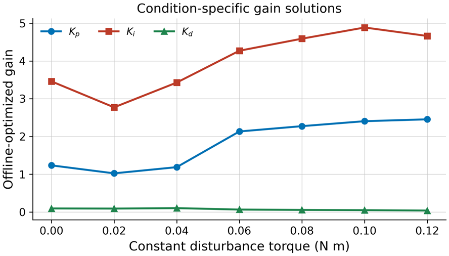
Figure 2 shows that the local solutions do not justify a simple monotonic gain schedule. K_i falls from 3.4604 at 0 N·m to 2.7725 at 0.02 N·m, then rises to 4.8866 at 0.10 N·m before decreasing at 0.12 N·m.

tu_pian_2.png

Figure 2. Condition-specific offline gain solutions for seven constant torques

Table 3 confirms that all seven local solutions remain inside the specified gain bounds. Settling time improves markedly relative to manual tuning, but no single gain varies monotonically with torque over the full range. The result is therefore evidence for the selected finite set of constrained optima.

Table 3. Seven-level condition-specific gain and performance results

4.2 Baseline and cross-condition tests

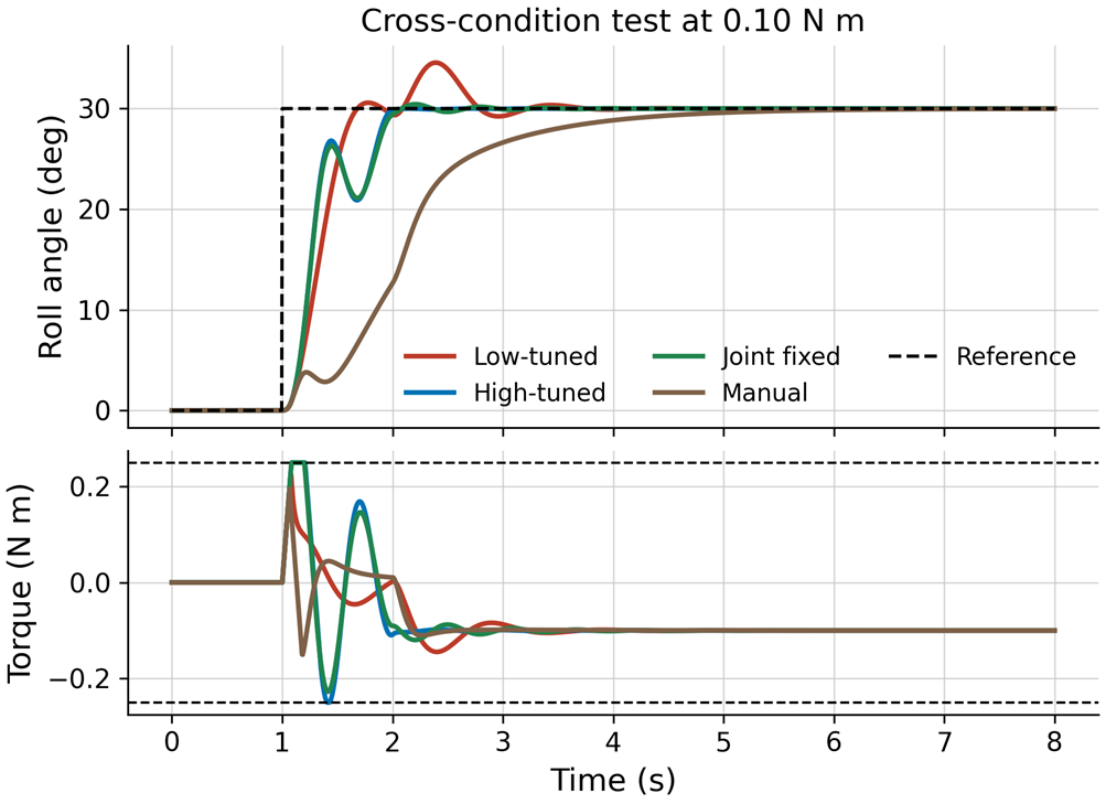
The joint fixed PID lowers IAE by 68.2% relative to the manual gains at 0.10 N·m and settles 2.63 s sooner, while remaining close to the condition-specific optimum. Table 4 summarizes the performance of the controller.

Figure 3 shows the cross-condition test response of roll angle and torque. It is observed that torque reaches the peak value of 0.25 N·m, but the integral state remains bounded because back-calculation is active.

Table 4. Performance at constant torque ${{\tau }_{d}}$ = 0.10 N·m

tu_pian_3.png

Figure 3. Cross-condition roll angle and applied torque at 0.10 N·m

Summary in Table 5 shows that the low-level gains are acceptable at 0.02 N·m but overshoot by 4.566 deg when tested at 0.10 N·m. The high-level gains and joint fixed gains remain stable at both conditions. Thus, the experiments show that a fixed controller should be tuned over the intended operating envelope for optimal results.

Table 5. Cross-condition robustness summary

4.3 Changing and nonconstant disturbances

Figure 4 shows the response of the controller to switching disturbances. With no gain updates during the run, the joint fixed PID returns to within ±0.6 deg of the 30 deg command in 0.485 s after the first 0.02 N·m step. The manual controller has not reached the same recovery band before the next event. Figure 5 shows roll angle variations of the joint-fixed PID controller to various input conditions and the results are summarized in Table 6. Across pulse, sinusoidal, and bounded stochastic tests, the joint controller remains bounded; IAE is 0.2370, 0.2911, and 0.2581 rad·s, respectively. A single settling-time value is not reported for the persistent sinusoid because the disturbance prevents permanent entry into a 2% band.

tu_pian_4.png

Figure 4. Response of one fixed controller to a 0.02-0.10-0.02 N·m torque sequence

tu_pian_5.png

Figure 5. Joint fixed-proportional-integral-derivative (PID) responses under pulse, sinusoidal, and stochastic torque

Table 6. Dynamic-profile performance of the joint fixed controller

4.4 Plant-parameter sensitivity

To test whether the fixed gains depend critically on the nominal coefficients, roll inertia J_x and viscous damping b are varied independently by ±20%, producing a 3 ´ 3 grid of nine plants. The controller gains, 0.10 N·m constant disturbance, actuator limits, integration step, and all metric definitions remain unchanged. This is a local parametric sensitivity test; it is not a substitute for identifying a physical airframe. Figure 6 shows the joint fixed PID controller sensitivity to inertia and damping and results are summarized in Table 7.

tu_pian_6.png

Figure 6. Roll response envelope for nine inertia-damping combinations at 0.10 N·m

Table 7. Joint fixed-proportional-integral-derivative (PID) sensitivity to inertia and damping

All nine responses remain bounded and converge to the reference. The slowest case occurs at 1.2 J_x and 0.8 b, where settling time rises to 2.82 s, overshoot to 2.907 deg, and IAE to 0.2431 rad·s. Lower inertia produces faster responses but approximately 1.27-1.45 deg overshoot. The nominally tuned fixed controller is therefore locally robust to the tested coefficient changes, although performance degrades as expected for larger inertia combined with weaker damping.

4.5 Aggregate performance and actuator use

A controller selected for an operating envelope should be judged across that envelope rather than at its best single point. Table 8 therefore aggregates the seven constant-torque tests. Relative to manual tuning, the joint fixed controller reduces mean settling time from 3.871 to 1.462 s and mean IAE from 0.6612 to 0.2048 rad·s. Its worst IAE is 0.2165 rad·s, which is only 8.7% above the worst condition-specific value of 0.1991 rad·s. The small loss relative to seven separate optima is the price of retaining one implementable gain vector.

The joint controller uses more control energy than the manual gains because it corrects the step and load changes more rapidly: mean E_u rises from 0.0340 to 0.0539 N²·m²·s.

Table 8. Aggregate results over seven constant-torque tests

4.6 Local linear stability check

A simple analytical check complements the time-domain simulations. If derivative filtering, saturation, rate limiting, and anti-windup are temporarily neglected, the ideal PID and reduced plant yield the characteristic polynomial

J_xs³+(b+K_d)s²+K_ps+K_i=0       (4)

For positive coefficients, the third-order Routh-Hurwitz condition is (b + K_d) K_p > J_x K_i. Define the normalized margin ρ = (b + K_d) K_p/(J_x K_i), for which ρ > 1 indicates local asymptotic stability in this idealized model. The joint fixed gains give ρ = 2.576. Across the seven condition-specific solutions, ρ ranges from 2.362 to 2.883. Thus, every reported gain vector passes the same local check with a finite margin.

This calculation is deliberately limited: it neither proves stability of the constrained nonlinear implementation nor establishes robustness beyond the tested plant set. The filtered derivative adds a state, while saturation, torque-rate limiting, and anti-windup make the closed loop piecewise nonlinear. The bounded disturbance tests, nine-plant parameter sweep, and step-size refinement therefore remain the primary numerical evidence.

4.7 Numerical and assumption audit

Table 9 records the status and role of every parameter that materially affects the reported response. These values define a reproducible benchmark.

Table 9. Status of constructed model and controller parameters

Table 10. Fixed-step refinement at 0.10 N·m

A step-size refinement check is also performed, as shown in Table 10 at the 0.10 N·m test using the joint fixed gains. Halving the nominal step from 0.005 to 0.0025 s changes IAE from 0.19762 to 0.19891 rad·s (0.65%) and overshoot from 0.434 to 0.411 deg. Doubling the step to 0.010 s gives the same 1.00 s settling time.

4.8 Interpretation relative to prior work

The simulations conducted support that tuning at one load can transfer poorly, while one fixed controller optimized over the intended envelope can remain consistent for the tested reduced-order plant than adaptive, estimator-based, or nonlinear quadrotor studies [10-17]. The main methodological contribution is consequently reproducibility.

4.9 Limitations and interpretation

This is a simulation-based control study with a focus on single axis stabilization with ± independent 20% variations of inertia and damping being tested and correlated. Pitch, yaw and other variations will be studied further and communicated in future articles.

We thank BNM Institute of Technology for providing facilities for using the MATLAB tool.