Riky Dwi Puriyanto* | Nuryono Satya Widodo | Haris Imam Karim Fathurrahman | Efa Wakhidatus Solikhah
© 2026 The authors. This article is published by IIETA and is licensed under the CC BY 4.0 license (http://creativecommons.org/licenses/by/4.0/).
OPEN ACCESS
Differential drive mobile robots (DDMRs) have been implemented in various applications to assist human work. One of the capabilities applied to DDMR to avoid collisions is obstacle avoidance. One approach used in the obstacle avoidance method is the sensor-based method. Sensor-based methods rely on sensory data to react to obstacles in real time. They are simple to implement and can handle dynamic environments effectively. This study aims to design an obstacle avoidance method using local sensors installed on the robot. The robot is designed to move according to the kinematic equations of DDMR. The results of this study indicate that the modification of the DDMR's kinematic equation that adds parameter c to the calculation of the robot's heading based on the results of ultrasonic sensor readings has been successfully applied to the obstacle avoidance function. DDMR can avoid obstacles in circles, lines, and U-shaped. The parameter c and instantaneous center of curvature (ICC) values significantly affect DDMR in producing trajectories when avoiding obstacles. The larger the c and ICC values, the more likely the robot is to move towards the negative y-axis, resulting in a greater DDMR distance to the goal.
differential drive mobile robots, obstacle avoidance, kinematic equation, local sensor-based, ultrasonic
Differential drive mobile robots (DDMRs) have become a widely adopted platform in autonomous robotic systems due to their simple mechanical design, high maneuverability, and relatively low implementation cost [1-3]. These characteristics make DDMRs particularly suitable for indoor service and logistics applications [4]. In modern warehouse environments, DDMRs are commonly deployed as autonomous mobile units responsible for tasks such as material transportation, sorting, and inventory handling [5]. Their differential drive configuration enables efficient motion csontrol and allows the robot to navigate through narrow corridors and cluttered indoor environments [6]. As a result, DDMR-based systems have been extensively utilized to improve operational efficiency, reduce labor costs, and increase the reliability of automated logistics operations.
Despite these advantages, autonomous navigation remains a fundamental challenge in mobile robotics. A key component of autonomous navigation is path planning [7-9], which aims to determine a feasible trajectory from an initial position to a desired target while satisfying several constraints, including obstacle avoidance [10], path efficiency [11], and energy consumption [12]. In real-world environments, this problem becomes significantly more complex due to environmental uncertainties such as dynamic obstacles, unexpected disturbances, and sensor noise. Furthermore, environments containing narrow passages, cluttered objects, or local minimum conditions can degrade the performance of conventional navigation algorithms. Consequently, robust path planning and obstacle avoidance strategies are essential to ensure safe, efficient, and reliable robot navigation [13].
Path planning methods in mobile robotics are generally categorized into global and local approaches [14]. Global path planning aims to compute an optimal path from the start position to the goal using a priori knowledge of the environment, typically represented as a map [15]. Classical graph-based algorithms such as A* and Dijkstra are widely used to generate optimal routes by considering obstacle locations and path length [16]. The primary advantage of global planning lies in its ability to produce globally optimal trajectories over long distances [17]. However, these methods generally rely on static environmental representations and therefore exhibit limited adaptability when unforeseen obstacles appear after the path has been generated.
In contrast, local path planning focuses on real-time navigation by utilizing information obtained from onboard sensors [18]. Local planners continuously adjust the robot trajectory according to its immediate surroundings, enabling responsive navigation in dynamic and uncertain environments [19]. However, local planning methods may suffer from several limitations, including oscillatory motion, inefficient trajectories, and the risk of becoming trapped in local minima [20]. These issues highlight the need for carefully designed local navigation strategies that can maintain stable and reliable motion behavior.
Within the context of local navigation, obstacle avoidance is a critical component that prevents collisions between the robot and surrounding objects. Existing obstacle avoidance approaches can generally be categorized into three main groups: sensor-based methods, behavior-based methods, and planning-based methods [21, 22]. Sensor-based methods rely directly on measurements obtained from onboard sensors such as ultrasonic sensors, LiDAR, or cameras to detect nearby obstacles [23-25]. These approaches allow robots to react rapidly to environmental changes and are relatively straightforward to implement in real-world robotic systems.
Behavior-based approaches decompose navigation into multiple reactive behaviors, such as goal seeking and obstacle avoidance. Representative techniques in this category include potential field methods, the vector field histogram, and wall-following strategies [26, 27]. These methods are attractive because they offer simplicity, robustness, and real-time responsiveness. However, they may exhibit undesirable behaviors such as oscillations or instability, particularly in environments with complex obstacle configurations.
Planning-based approaches, on the other hand, generate collision-free trajectories through explicit path optimization or graph-search processes. Representative examples include graph-based algorithms such as A* and Dijkstra, as well as sampling-based techniques such as rapidly exploring random trees (RRTs) and Probabilistic Roadmaps [28, 29]. Although these methods can produce efficient trajectories in structured environments, they typically require significant computational resources and may have limited responsiveness to rapidly changing environments.
Despite the extensive research on obstacle avoidance, several challenges remain. Sensor-based and behavior-based approaches provide fast and reactive navigation but may produce unstable or suboptimal trajectories. Conversely, planning-based approaches can provide more optimal solutions but generally require higher computational effort and depend on explicit environmental models. Therefore, there remains a need for navigation strategies that preserve the simplicity and responsiveness of sensor-based approaches while improving trajectory stability and heading control.
Motivated by this challenge, this study proposes an obstacle avoidance strategy based on a modification of the kinematic model of a differential drive mobile robot. In the proposed approach, sensor measurements obtained from local sensors are incorporated to influence the robot heading during navigation. Specifically, a modification is introduced into the conventional DDMR kinematic model by incorporating an additional parameter that adjusts the robot heading when obstacles are detected in front of the robot. This modification enables the robot to adapt its motion in real time while maintaining stable navigation behavior. Consequently, the proposed approach aims to improve trajectory stability and obstacle avoidance performance while preserving the computational simplicity required for real-time implementation.
2.1 Obstacle avoidance in kinematics of DDMR
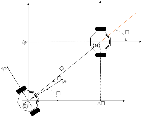
The study utilizes the kinematic model of the DDMR to generate robot motion. According to Figure 1, the DDMR moves from the initial position {I} to the target/goal position {G}. The robot moves on a Cartesian plane along the x and y coordinates. Changes in position on each axis and the robot's facing angle can be seen in Eqs. (1)-(3).
$\dot{x}=v \cos \theta$ (1)
$\dot{y}=v \sin \theta$ (2)
$\dot{\theta}=\omega$ (3)
Figure 1. Parameters of DDMRs
The movement of the robot's position from {I} to {G} is represented by ρ. According to Eq. (4), ρ is the Euclidean distance between the current and target positions. The difference between the x and y coordinates of the robot at the current position and its previous position on the Cartesian plane are represented as Δx and Δy. The angle change generated by DDMR to frame {I} generated by the gyroscope is represented by θ. In Eq. (5), the resulting angle difference in the condition {I} to {G} is represented by α. The resulting final angle to the DDMR frame is defined by β at the goal position.
$\rho=\sqrt{\Delta x^2+\Delta y^2}$ (4)
$\alpha=\left(\tan ^{-1}\left(\frac{\Delta y}{\Delta x}\right)+c\right)-\theta$ (5)
$\beta=-\theta-\alpha$ (6)
The kinematic equation of DDMR is modified by adding a constant value (c) in Eq. (5). The value of c is a positive constant influencing the robot's heading angle. The value of c is determined by the position of the obstacle detected by the sensor installed on the robot. Eqs. (4)-(6) are used to produce the robot's linear velocity ( ) and angular velocity (
 ) shown in Eqs. (7) and (8).
$v=k_\rho \rho$ (7)
$\omega=k_\alpha \alpha+k_\beta \beta$ (8)
$k_\alpha, k_\rho$, and $k_\beta$ are gain parameters that make DDMR achieve stability at the goal position. The control law that applies so that DDMR reaches the goal position is $k_\rho>0, k_\beta<$ 0 , and $k_\alpha-k_\beta>0$. Based on Eqs. (7) and (8), the speed of the left $\left(v_l\right)$ and right $\left(v_r\right)$ motors is set according to Eqs. (9) and (10). The value of L is the distance between the right and left wheels of the DDMR. The parameter R is the instantaneous center of curvature (ICC) of the DDMR.
$v_r=v+\frac{\omega L}{2 R}$ (9)
$v_l=v-\frac{\omega L}{2 R}$ (10)
To improve the clarity of the proposed navigation strategy, the overall procedure of the obstacle avoidance method is summarized in Algorithm 1. The algorithm describes how sensor measurements are incorporated to modify the robot heading during navigation while maintaining the kinematic constraints of the differential drive mobile robot.
|
Algorithm 1: Sensor-Based Obstacle Avoidance |
|
|
Input: Current robot pose ($x, y, \theta$) Goal position (xg, yg) Distance sensors SL, SC, SR Control gains $k_\rho, k_\alpha, k_\beta$ Robot parameters L, R Constant c |
|
|
Output: Wheel velocities $v_r, v_l$ |
|
|
1 |
$\Delta x \leftarrow x_g-x$ |
|
2 |
$\Delta y \leftarrow y_q-y$ |
|
3 |
// Lookup table for angular offset |
|
4 |
LUT ← [0, c, c, 2c, −c, −2c, c, 2c] |
|
5 |
c_offset ← LUT |
|
6 |
// Navigation variable |
|
7 |
$\rho \leftarrow \sqrt{\Delta x^2+\Delta y^2}$ |
|
8 |
$\alpha \leftarrow\left(\tan ^{-1}\left(\frac{\Delta y}{\Delta x}\right)+c\right)-\theta$ |
|
9 |
$\beta \leftarrow-\theta-\alpha$ |
|
10 |
// Control law |
|
11 |
$v \leftarrow k_\rho \rho$ |
|
12 |
$\omega \leftarrow k_\alpha \alpha+k_\beta \beta$ |
|
13 |
// Wheel velocities |
|
14 |
$v_r \leftarrow v+\frac{\omega L}{2 R}$ |
|
15 |
$v_l \leftarrow v-\frac{\omega L}{2 R}$ |
|
16 |
return $v_r, v_l$ |
2.2 Robot design
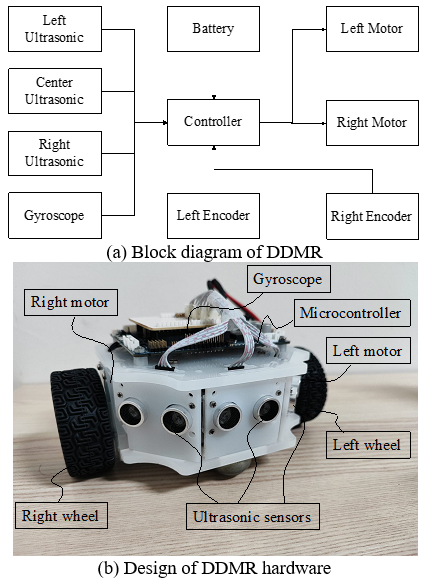
Based on the explanation in the previous section, this study uses a differential drive-based mobile robot. DDMR consists of several components according to the design of the block diagram and hardware in Figure 2(a) and (b). The robot consists of a microcontroller as a robot controller. The microcontroller receives input data from sensors installed on the robot. Information from the sensors will be processed, and the computational results will be used to regulate the speed of the right and left motors.
The sensors used in DDMR measure distance, motor speed, and robot rotation angle. The distance sensors used are ultrasonic-based, totaling three. In this study, ultrasonic sensors were installed on the robot's left, middle, and right sides. The motor speed sensor was made of internal encoders of the right and left motors. The gyroscope was used as the robot angle counter. The robot's facing angle information from the gyroscope replaces Eq. (3). This reduces errors in determining the robot's facing angle compared to using encoder data.
Figure 2. Design of differential drive mobile robots (DDMR)
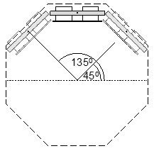
The obstacle avoidance method, based on local sensors on the robot, is designed using ultrasonic sensors. The design of the distance sensor used in real-time detection of obstacles can be seen in Figure 3. Three sensors are installed on the front of the robot with a 45° angle difference between sensors. The three sensors are 0.065 m from the center of the robot. This will determine the robot's safe distance to avoid collisions with obstacles.
Figure 3. Design of three ultrasonic sensors
Based on Figure 3, three ultrasonic sensors are used to determine the position of obstacles to the robot. This is used to determine the value of c in Eq. (5). Table 1 shows the relationship between the positions of obstacles represented through the conditions of the sensors that detect objects. The lookup table method is used to determine the value of c. Condition 1 indicates the sensor when it detects an obstacle in front. Vice versa, condition 0 represents the sensor when it does not detect an obstacle in front. This condition is determined by the safe distance value between the robot and the obstacle determined at the beginning.
Table 1. Condition of each sensor
|
Condition of Sensor |
Value of c |
||
|
Left |
Center |
Right |
|
|
0 |
0 |
0 |
0 |
|
0 |
0 |
1 |
c |
|
0 |
1 |
0 |
c |
|
0 |
1 |
1 |
2c |
|
1 |
0 |
0 |
-c |
|
1 |
0 |
1 |
-2c |
|
1 |
1 |
0 |
c |
|
1 |
1 |
1 |
2c |
The coordinates of the position headed by the robot will be affected by the reading results of the distance sensor installed on the robot. Based on the distance sensor detection results, the speed values of the right and left motors will change from the calculation of the standard kinematic equation. The robot will recalculate the next position according to the applicable DDMR's kinematic equation until it reaches the target.
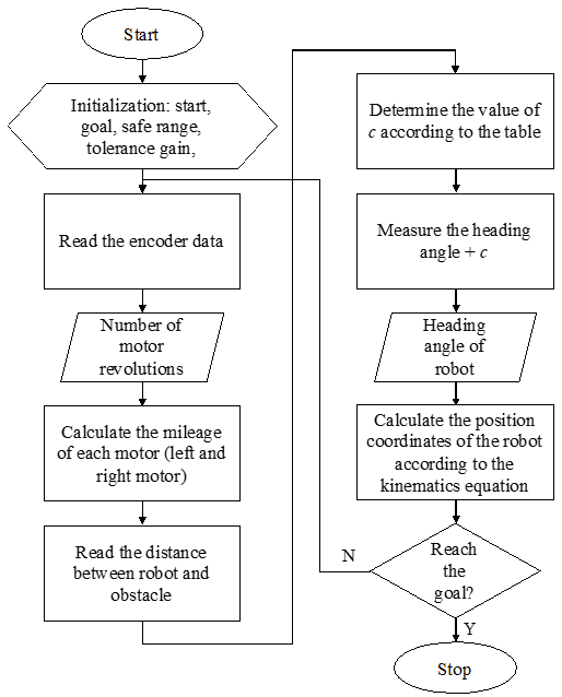
In general, the DDMR process moves from the initial to the goal position while avoiding obstacles in between, as can be seen in Figure 4. Initialization needs to be done by determining the initial position, goal position, the safe distance of the robot to obstacles, and the error tolerance to the goal position. In addition, the gain value involved in the DDMR kinematic equation must be defined at the beginning. After that, the encoder data on each motor is converted into the distance traveled and entered into the DDMR kinematic equation.
Figure 4. Flowchart of robot movement in reaching the target
The robot position is obtained based on the DDMR kinematics calculation. Based on the target position, the speed values of the right and left motors are determined according to Eqs. (9) and (10). When the DDMR encounters an obstacle between the DDMR and the goal position, the value of c is determined based on Table 1. This will affect the robot heading, which will be measured using a gyroscope installed on the DDMR. The DDMR will continue to move until it reaches the target. When the DDMR has not reached the goal position, the DDMR will search for the following position coordinates to reach the target.
3.1 Influence of gain parameter on DDMR trajectory
In the study, DDMR navigates according to kinematic equations, such as Eqs. (1)-(10). The linear velocity (v) and angular velocity ( $\omega$ ) are highly influenced by the gain values of $k_\alpha$ and $k_\rho$. Following the control law, DDMR was able to reach the goal when the values of $k_\alpha$ and $k_\rho$ are positive. The influence of $k_\alpha$ value in the movement of DDMR can be observed in Figure 5. DDMR moved from the initial coordinate position $(0,0)$ to the goal coordinate position $(10,10)$ with the values of $k_\alpha$ and $k_\rho=0.1$, and the initial heading angle $\left(\theta_i\right)=1.57 \mathrm{rad}$.

Figure 5. Influence of $k_\alpha$ value on the trajectory of DDMRs

Figure 6. The influence of $k_\rho$ values on the trajectory of DDMRs
Based on Figure 5, the path resulted from the movement of DDMR with the value of $k_\alpha=1$ was further than that of bigger $k_\alpha$ values. A bigger value of $k_\alpha$ resulted in a trajectory that was closer to the target; the resulting path will resemble a straight line with a big value of $k_\alpha$. This can be seen with $k_\alpha$ $=100$ that resulted in a straight path toward the target.
The value of $k_\rho$ determines the length of steps used each time to move from $q_t$ to $q_{t+1}$. A big value of $k_\rho$ resulted in big steps; conversely, a small value of $k_\rho$ makes the robot move in smaller steps. Thus, the use of $k_\rho$ with smaller values require a longer time to reach the target. The influence of $k_\rho$ values can be seen in Figure 6.
3.2 Implementation of obstacle avoidance algorithm
Based on the evaluations above, the gain parameter values of $k_\rho, k_\alpha$ and $k_\beta$ used to evaluate the DDMR were 0.1, 20, and -0.01, respectively. The subsequent evaluation assessed the proposed method's effectiveness in avoiding obstacles. In this study, the obstacle avoidance performance is evaluated using three representative obstacle configurations: circular, line-shaped, and U-shaped obstacles. These configurations are selected because they capture fundamental geometric characteristics commonly encountered in indoor navigation environments while allowing a systematic evaluation of the robot’s reactive navigation behavior. Circular obstacles represent isolated objects that require the robot to perform smooth trajectory deviations and subsequently reorient toward the target. Line-shaped obstacles emulate walls or extended barriers, which are useful for assessing heading stability and the robot’s ability to maintain safe distances from continuous boundaries. Meanwhile, U-shaped obstacles are widely used to evaluate the robustness of obstacle avoidance strategies in the presence of potential local minima, where purely reactive algorithms may become trapped or exhibit oscillatory motion. By employing these three obstacle types, the experiments can comprehensively assess the robot’s capability to handle isolated obstacles, extended barriers, and trapping structures. More complex scenarios such as narrow passages are not considered in this evaluation because they primarily test precision navigation and global path planning capabilities rather than the fundamental reactive obstacle avoidance behavior that constitutes the main focus of this study. In the first evaluation, a tube-shaped obstacle with a radius of 0.05 m and a height of 0.25 m was placed between the robot and the target. The test was conducted in a closed and conditioned room measuring 3 m × 3 m with a flat floor. The results of the evaluation can be seen in Figures 7 and 8.
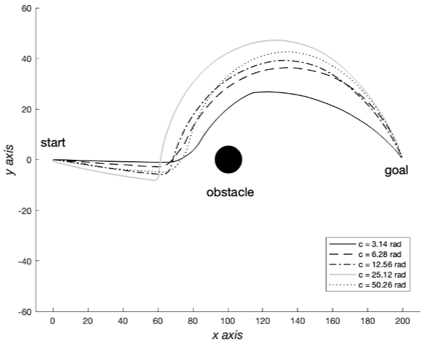
Figure 7 shows the resulting trajectory of DDMR, referring to the proposed modification of the kinematic equations. In the evaluation, DDMR moved from the initial position (0,0) toward the goal position (200,0) in centimeter units. A central obstacle in tubular shape was placed at the position of (100,0) with a radius of 0.05 m. Besides, the ICC value influencing the speed of right and left motors, as in Eqs. (9) and (10), was 1 m. The safe distance of the robot against the obstacle (r), measured by the ultrasonic sensor, was 0.45 m. The evaluation aims to observe the influence of the c value proposed in Eq. (5) concerning obstacle avoidance. As shown in Figure 7, the proposed change of c values made the robot successfully avoid the tube-shaped obstacle that was placed in front of the robot. The value of c is the heading angle value added to the kinematic equation, influenced by the sensor reading. In the first evaluation, five values of c were used to observe the effectiveness of the obstacle avoidance function: 3.14 rad, 6.28 rad, 12.56 rad, 25.12 rad, and 50.26 rad. Overall, a bigger value of c influences the trajectory of DDMR, resulting in wider trajectories. This influences the travel distance of DDMR in reaching the goal position. As seen in Table 2, the travel distance with the setting of a big value of c tends to be further than that of a small value of c. Besides, a bigger c value tends to sharpen the maneuver of DDMR during the initial period of obstacle avoidance.
Figure 7. The influence of the c parameter on the trajectory of DDMRs with a tube-shaped obstacle
Figure 8. Various distance values between the DDMRs and the obstacle due to changing values of c
Table 2. Result of experiment 1
|
n |
Value of c (rad) |
Time to Goal (s) |
Mileage (m) |
Minimum Distance to Obstacle (m) |
|
1 |
3.14 |
135 |
0.210 |
0.16 |
|
2 |
6.28 |
134 |
0.227 |
0.23 |
|
3 |
12.56 |
136 |
0.230 |
0.26 |
|
4 |
25.12 |
140 |
0.250 |
0.36 |
|
5 |
50.24 |
134 |
0.236 |
0.23 |
Figure 8 shows the comparison of safe distance traveled by DDMR during the first evaluation. The safe distance of DDMR toward the obstacle was determined at 0.35 m. As in Figure 8, trajectory with the value of c = 25.12 displays the safest value among other trajectories. As in Table 2, the minimum safest distance of DDMR toward the obstacle was found at the value of c = 25.12. As the value of c becomes greater than 25.12, the value of the minimum distance between the DDMR and the obstacle becomes smaller.
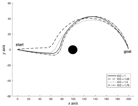
The second experiment was conducted in the same environment as the first experiment. The second evaluation was performed to observe the influence of ICC on the trajectory of DDMR in the function of obstacle avoidance. The ICC values used in the evaluation were 1.00, 1.25, 1.5, and 1.75. The change of the ICC values affects the maneuver of DDMR when making turns. As in Figure 9, a bigger value of ICC sharpens the maneuver of DDMR when avoiding the obstacle. This also impacts the travel distance of DDMR when reaching the goal position.
Figure 9. The influence of the ICC parameter on the trajectory of DDMRs with a tube-shaped obstacle
According to Figure 10, the modification of ICC values generally affects the maneuver in avoiding obstacles within the initial period. Based on Table 3, the value of ICC = 1.25 generated the greatest amount of minimum distance toward the obstacle. This was caused by the speedy maneuver of DDMR during the initial period when the ultrasonic sensor detected the obstacle. With the value of ICC equal to 1.75, the value of safe minimum distance toward the obstacle was the smallest among other values of ICC. This occurred due to the initial movement of DDMR along the y-axis before detecting the obstacle was negative. DDMR performed the sharp maneuver when detecting the obstacle; however, the initial movement made the minimum distance toward the obstacle become the smallest among other values. Besides, the travel distance of the DDMR toward the goal position was the greatest with the setting value of ICC = 1.75.
Figure 10. The distance of DDMRs in regard to the obstacle due to the changing values of ICC
Table 3. Results in experiment 2
|
n |
Value of c (rad) |
Time to Goal (s) |
Mileage (m) |
Minimum Distance to Obstacle (m) |
|
1 |
1.00 |
134 |
0.236 |
0.23 |
|
2 |
1.25 |
133 |
0.227 |
0.32 |
|
3 |
1.50 |
134 |
0.229 |
0.26 |
|
4 |
1.75 |
135 |
0.237 |
0.21 |
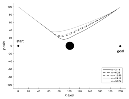
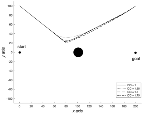
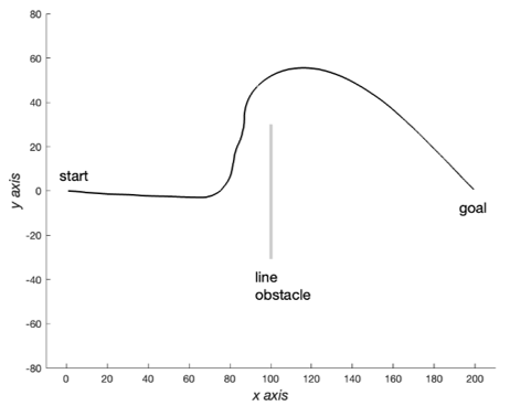
A more complex evaluation was conducted with the line-based obstacles. The third and fourth evaluations were conducted on the obstacles with straight-line and U-shaped obstacles. In the third evaluation, the DDMR faced a line-shaped obstacle with a length of 0.63 m, positioned vertically aligned with y-axis, in between the initial and the goal position. The trajectory results of the DDMR encountering a straight-line obstacle can be seen in Figure 11. According to Table 1, the DDMR will generate an additional steering angle of 2c. Therefore, when the DDMR is in front of a linear obstacle with all ultrasonic sensors detecting it, the DDMR will maneuver toward the positive y-axis. The evaluation with the line-shaped obstacle utilized the parameter values of c = 25.12 and ICC = 0.5. The travel time required by the DDMR to achieve the goal position was 133 s, while the travel distance was 0.254 m.
Figure 11. The influence of the ICC parameter on the trajectory of DDMRs with a line-shaped obstacle
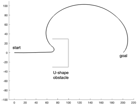
Figure 12. The influence of the ICC parameter on the trajectory of DDMRs with the U-shaped obstacle
The evaluation of DDMR with a U-shaped obstacle can be seen in Figure 12. The evaluation on the U-shaped obstacle utilized c = 12.56 and ICC = 1.25. The travel time required by the DDMR to achieve the goal position was 165 s, while the travel distance required was 0.367 m.
This study demonstrates that the proposed modification of DDMR’s kinematic equations, incorporating the parameter c into the heading calculation based on ultrasonic sensor readings, effectively enhances obstacle avoidance. The algorithm enables the robot to successfully navigate circular, line, and U-shaped obstacles. Quantitative results indicate that the parameters c and ICC critically influence trajectory generation and travel distance, and their appropriate selection can optimize obstacle avoidance performance. These findings highlight the effectiveness and practical applicability of the proposed approach, providing a robust framework for real-time autonomous navigation in complex environments.
[1] Vesentini, F., Rigo, D., Sansonetto, N., Di Persio, L., Muradore, R. (2024). Minimum-energy switching geometric filter on Lie groups for differential-drive wheeled mobile robots. European Journal of Control, 80: 101101. https://doi.org/10.1016/j.ejcon.2024.101101
[2] Balbuena, J., Sinche, J., Quiroz, D., Arce, D., Villota, E. (2026). PlatROB: An open-source, modular, and low-cost hardware platform for mobile robotics and AI education. HardwareX, 25: e00747. https://doi.org/10.1016/j.ohx.2026.e00747
[3] Rosenfelder, M., Carius, H., Herrmann-Wicklmayr, M., Eberhard, P., Flaßkamp, K., Ebel, H. (2025). Efficient avoidance of ellipsoidal obstacles with model predictive control for mobile robots and vehicles. Mechatronics, 110: 103386. https://doi.org/10.1016/j.mechatronics.2025.103386
[4] Kardas, P., Bielecb, F., Braun, M., et al. (2025). Evaluation of disinfection methods for autonomous mobile robots used in hospital logistics in emergency departments. Journal of Hospital Infection, 162: 17-25. https://doi.org/10.1016/j.jhin.2025.05.006
[5] Zhou, X.M. (2026). Optimization of DDPG positioning and navigation technology for warehouse logistics robots. Progress in Engineering Science, 3(2): 100229. https://doi.org/10.1016/j.pes.2026.100229
[6] Castri, L., Beraldo, G., Bellotto, N. (2026). Causality-enhanced decision-making for autonomous mobile robots in dynamic environments. Expert Systems with Applications, 309: 131246. https://doi.org/10.1016/j.eswa.2026.131246
[7] Luo, Y., Jia, B.X., Bai, Z.H., et al. (2025). Path planning for orchard mobile robots based on an improved ant colony algorithm and the dynamic window approach. Smart Agricultural Technology, 12: 101518. https://doi.org/10.1016/j.atech.2025.101518
[8] An, Z.H., Li, C.Y., Han, Y., Niu, M.R. (2025). Improved bidirectional JPS algorithm for mobile robot path planning in complex environments. Computers, Materials & Continua, 83(1): 1347-1366. https://doi.org/10.32604/cmc.2025.059037
[9] Ye, F., Duan, P., Meng, L.L., Xue, L.Y. (2025). A hybrid artificial bee colony algorithm with genetic augmented exploration mechanism toward safe and smooth path planning for mobile robot. Biomimetic Intelligence and Robotics, 5(2): 100206. https://doi.org/10.1016/j.birob.2024.100206
[10] Yuan, X.Y., Wang, J.W., Tong, C.C., Wang, H.B. (2025). Integrated path planning for AUV communication efficiency and obstacle avoidance based on ant colony optimization and three-dimensional dynamic window algorithm. Applied Ocean Research, 156: 104465. https://doi.org/10.1016/j.apor.2025.104465
[11] Zhong, J.K., Kong, D.Y., Wei, Y.L., Hu, X.J., Yang, Y. (2025). Efficiency-optimized path planning algorithm for car-like mobile robots in bilateral constraint corridor environments. Robotics and Autonomous Systems, 186: 104923. https://doi.org/10.1016/j.robot.2025.104923
[12] Gao, L.F., Wang, W.D., Ke, D.Y. (2025). Energy optimization for autonomous mobile robot path planning based on deep reinforcement learning. Computers, Materials & Continua, 86(1): 1-15. https://doi.org/10.32604/cmc.2025.068873
[13] Karthikeyan, R., Sheela Rani, B. (2025). An innovative approach for obstacle avoidance and path planning of mobile robot using adaptive deep reinforcement learning for indoor environment. Knowledge-Based Systems, 326: 114058. https://doi.org/10.1016/j.knosys.2025.114058
[14] Tao, Y.H., Du, J.L. (2025). Time-optimal global path planning and collision-avoidance local path planning for USVs in traffic separation scheme-implemented coastal waters. ISA Transactions, 165: 280-294. https://doi.org/10.1016/j.isatra.2025.06.030
[15] Yuan, L.W., Luo, J.W. (2025). Approach to global path planning and optimization for mobile robots based on multi-local gravitational potential fields bias-P-RRT*. Journal of Computational Science, 92: 102718. https://doi.org/10.1016/j.jocs.2025.102718
[16] Masing, B., Lindner, N., Bortoletto, E. (2025). Computing all shortest passenger routes with a tropical Dijkstra algorithm. EURO Journal on Transportation and Logistics, 14: 100163. https://doi.org/10.1016/j.ejtl.2025.100163
[17] Feng, C.L., Zhang, Q., Wang, J.X., et al. (2026). Excavator trajectory planning via global probabilistic learning from expert demonstrations. Automation in Construction, 182: 106736. https://doi.org/10.1016/j.autcon.2025.106736
[18] Ben-Akka, M., Tanougast, C., Diou, C. (2025). Novel design of reward and epsilon-greedy decay strategy tailored for Q-learning in optimizing local mobile robot path planning. Knowledge-Based Systems, 324: 113836. https://doi.org/10.1016/j.knosys.2025.113836
[19] Shareef, A., Al-Darraji, S., Al-Ansarry, S., et al. (2025). Local path planning based on Bi-population swarms optimization algorithms. Results in Control and Optimization, 21: 100634. https://doi.org/10.1016/j.rico.2025.100634
[20] Xu, J.L., Peng, X.C., Chen, M. (2026). Memory-based iterated local search with multiple perturbation operators for personalized learning path planning. Applied Soft Computing, 188: 114426. https://doi.org/10.1016/j.asoc.2025.114426
[21] Wang, J.C., Yang, L.L., Cen, H.Y., He, Y., Liu, Y.F. (2025). Dynamic obstacle avoidance control based on a novel dynamic window approach for agricultural robots. Computers in Industry, 167: 104272. https://doi.org/10.1016/j.compind.2025.104272
[22] Ospina, R., Itakura, K. (2025). Obstacle detection and avoidance system based on layered costmaps for robot tractors. Smart Agricultural Technology, 11: 100973. https://doi.org/10.1016/j.atech.2025.100973
[23] Li, C.Y., Yang, Y.H., Huang, T.Y., Chen, X.B. (2025). A flocking robots round-up multi-target and obstacle avoidance control algorithm. Journal of the Franklin Institute, 362(16): 108111. https://doi.org/10.1016/j.jfranklin.2025.108111
[24] Chang, L., Shan, L., Zhang, W.L., Jiang, C., Wang, W.X., Dai, Y.W. (2025). A LiDAR and reasoning-based artificial potential field for mobile robot navigation in unknown and dynamic environments. Advanced Engineering Informatics, 67: 103519. https://doi.org/10.1016/j.aei.2025.103519
[25] Shalihan, M., Cao, Z., Lau, B.P.L., Liu, R., Yuen, C., Tan, U.X. (2025). MR-FLOUR: Multi-robot Relative localization based on the Fusion of LiDAR, Odometry, and UWB Ranging. Mechatronics, 112: 103410. https://doi.org/10.1016/j.mechatronics.2025.103410
[26] Li, M.H., Huang, Z.J., Bi, W.H., Hou, T.L., Yang, P., Zhang, A. (2025). A fish evasion behavior-based vector field histogram method for obstacle avoidance of multi-UAVs. Aerospace Science and Technology, 159: 109974. https://doi.org/10.1016/j.ast.2025.109974
[27] Zhu, J.R., Zhang, P.X., Zhu, Y.Q. (2024). CREST: A target-point-based wall-climbing robot capable of spatial traversal and obstacle avoidance. Results in Engineering, 24: 103638. https://doi.org/10.1016/j.rineng.2024.103638
[28] Pan, Q.Q., Wang, H.B., Feng, Y.F., Guo, S.J., Luo, J.J. (2026). RRT-based CPC: A configuration planning method for continuum robots using rapidly-exploring random tree algorithm. Robotics and Autonomous Systems, 195: 105190. https://doi.org/10.1016/j.robot.2025.105190
[29] Yang, H.J., Luo, X., Duan, C., et al. (2025). Research on multi-objective point path planning for mobile inspection robot based on multi-informed-rapidly exploring random tree∗. Engineering Applications of Artificial Intelligence, 151: 110645. https://doi.org/10.1016/j.engappai.2025.110645