Chenglin Yang | Xinyu Hao | Hua Jin*
© 2026 The authors. This article is published by IIETA and is licensed under the CC BY 4.0 license (http://creativecommons.org/licenses/by/4.0/).
OPEN ACCESS
Unmanned aircraft system (UAS) threats pose increasing security challenges to critical infrastructure, especially under low-frequency but high-consequence scenarios where historical data are limited. This study proposes a structured risk assessment and defensive resource prioritization framework based on the Target Loss Probability Model. An evaluation index system comprising Target Value (RV), Attacker Resource (RA), and Defensive Resources (RD) is constructed, and the Maximizing Deviation Method is used to integrate subjective and objective indicator weights under small-sample expert-scoring conditions. Monte Carlo simulation is applied to construct relative risk grading thresholds, while Sobol global sensitivity analysis is used to identify key defensive indicators. A scenario-based case study of an anonymized nuclear facility shows that increasing the defensive resource capability index from 0.5542 to 0.8245 reduces the Target Loss Probability index from 0.2542 to 0.2039, thereby downgrading the relative risk level from high to medium. The proposed framework transforms qualitative threat factors into computable model inputs and provides decision support for prioritizing improvements to counter-UAS RD.
counter-UAS defense, critical infrastructure, Maximizing Deviation Method, risk assessment, Target Loss Probability Model, unmanned aircraft system threats
With the rapid development and proliferation of unmanned aircraft system (UAS) technology, its applications in aerial photography, logistics, and agriculture have expanded rapidly. However, malicious UAS activities involving reconnaissance, smuggling, jamming, and direct attacks have increasingly challenged the security of critical infrastructure. Representative incidents include the 2019 drone attacks on Saudi Aramco facilities, the sustained use of loitering munitions against Ukraine’s power infrastructure since 2022, and the expansion of drone strikes against energy and industrial facilities since 2024 [1-3].
When facing UAS threats, low-altitude attacks against critical infrastructure and key assets may not only cause casualties and facility damage, but may also trigger secondary impacts through functional interdependencies among critical infrastructure systems. The Directive (EU) 2022/2557, namely the Critical Entities Resilience Directive (CER Directive), which formally entered into force in 2023, clearly defines the scope of critical entities and requires Member States and operators to conduct risk assessments based on an all-hazards approach [4].
Early risk assessments of UAS threats to critical infrastructure and key assets focused primarily on qualitative analysis and regulatory compliance. The European Union Aviation Safety Agency (EASA) has formulated guidance for UAS operational safety [5]. As UAS threat types diversified, quantitative approaches such as Multi-Criteria Decision Making (MCDM) models have been introduced into critical-infrastructure resilience and risk assessment [6], while data availability and data scarcity remain major challenges in critical-infrastructure modelling and risk assessment [7]. Therefore, the study introduces the Target Loss Probability Model into existing risk assessment approaches and uses it as a risk assessment function from an attacker-defender perspective. The model is used to calculate the Target Loss Probability index and to support the identification of defensive resource improvement priorities.
Although existing MCDM-based and expert-scoring methods provide useful tools for structuring complex risk indicators, most of them aggregate indicators through linear or quasi-linear weighting procedures. Such approaches are effective for ranking alternatives, but they have limited ability to represent the nonlinear interaction among attacker capability, defensive capability, and Target Value (RV) in UAS threat scenarios. Bayesian-network-based methods can describe probabilistic dependencies among risk factors, but they usually require prior probabilities and conditional probability tables, which are difficult to obtain for low-frequency but high-consequence UAS threats against critical infrastructure. Qualitative C-UAS risk assessment approaches are valuable for threat identification and operational guidance, but they often provide limited support for producing a computable risk index and for evaluating how changes in RD affect the overall risk level.
To address these limitations, this study introduces the Target Loss Probability Model as a nonlinear risk calculation function for UAS threat assessment of critical infrastructure and key assets. Compared with conventional MCDM-style indicator aggregation, the proposed framework does not simply sum weighted indicators into a general risk score. Instead, it explicitly couples RV, Attacker Resource (RA), and RD within a unified attacker–defender modeling structure. This makes it possible to transform qualitative UAS threat factors into normalized model inputs and to calculate a Target Loss Probability index under data-scarce and security-sensitive conditions. Furthermore, Monte Carlo simulation is used to construct relative risk-grading thresholds from the model output distribution, while Sobol global sensitivity analysis is introduced to identify the defensive indicators that contribute most to changes in the Target Loss Probability index. Therefore, the proposed framework extends traditional expert-scoring and MCDM approaches from static indicator aggregation to nonlinear risk calculation, risk-level interpretation, and defensive resource prioritization.
The main contributions of this study are threefold. First, this study develops a Target Loss Probability Model-based framework that links RA, RD, and RV through a nonlinear risk calculation mechanism, thereby extending conventional MCDM-style indicator aggregation. Second, it constructs a UAS threat-oriented indicator system for critical infrastructure by integrating attacker capability, defensive capability, and RV factors, and combines expert scoring with the Maximizing Deviation Method to obtain indicator weights under data-scarce conditions. Third, it integrates Monte Carlo-based risk grading and Sobol global sensitivity analysis to support both risk-level interpretation and sensitivity-based defensive resource prioritization.
2.1 Target Loss Probability Model
The Target Loss Probability Model, proposed by Major, is a mathematical model for risk assessment that is mainly used to describe the interaction among RV, RA, and RD [8]. In the context of UAS threats to critical infrastructure and key assets, this study uses the Target Loss Probability Model as a risk assessment function from an attacker–defender perspective. Here, the attacker–defender relationship refers primarily to the resource-based confrontation between hostile UAS actors and the counter-UAS defense system of critical infrastructure and key assets. The core objective is to use the Target Loss Probability Model to generate a computable risk index and further analyze how improvements in defensive resource capability affect risk reduction.
In this study, the model is mainly used to characterize the interaction among attack capability, defensive capability, and RV. For computational tractability, attack behavior is treated from the defender’s perspective as an external pressure under a given threat scenario, and the analysis focuses on the effect of changes in the defensive resource capability index on the Target Loss Probability index. Under this attacker-defender relationship, the attacker’s payoff is regarded as corresponding to the defender’s loss; the expected payoff/loss (EL) is expressed as follows [8]:
$E L=\sum_{i=1}^n V_i \cdot p\left(V_i, A_i, D_i\right)$ (1)
where, $V_i$, $A_i$ and $D_i$ denote the RV, and RD for the target $i$, respectively.
In this study, $V_i$ represents the intrinsic value, strategic importance, and potential consequence severity of critical infrastructure and key assets under UAS threat events. $A_i$ represents the comprehensive attack capability of hostile UAS actors in conducting threat activities, including personnel capability, technical capability, financial support, UAS platform performance, payload capability, intelligence planning capability, and coordinated penetration capability. $D_i$ represents the comprehensive defensive capability of critical infrastructure and key assets against UAS threats, including detection, identification, countermeasures, barriers, and management capabilities. On this basis, the Target Loss Probability Model can be expressed as:
$p=p\left(V_i, A_i, D_i\right)=\exp \left(-\frac{A_i \cdot D_i}{\sqrt{V_i}}\right) \times\left(\frac{A_i{ }^2}{A_i{ }^2+V_i}\right)$ (2)
where, $p\left(V_i, A_i, D_i\right)$ denotes the Target Loss Probability index.
It should be noted that this value is not an empirically observed attack occurrence probability derived from a large number of historical samples. Rather, it is a normalized risk index calculated from the RV, RA, and RD. This index is mainly used to compare relative changes in risk under different defensive states. In the subsequent case study, RV and RA are treated as given scenario conditions, while RD is regarded as the main adjustable variable. Therefore, the model-recommended defensive resource capability value calculated later should be interpreted as a model-based defensive capability target, which is used to guide the improvement of defensive capability.
2.2 Indicator system and quantification
2.2.1 Adaptability analysis of model elements
Factor consistency between the Target Loss Probability Model and traditional risk assessment frameworks forms the theoretical foundation for the proposed model's applicability. Traditional risk assessment theory generally centers on three core factors: Threat likelihood $(T)$, vulnerability $(V)$, and consequence severity $(C)$. By contrast, the Target Loss Probability Model employs RA $(A)$, RD $(D)$, and RV $(V)$ as input parameters [9]. Despite terminology differences, the two models exhibit structural isomorphism in risk transmission mechanisms: threat likelihood is reflected by the attacker's capability and intent; vulnerability mirrors the defender's performance in detection, delay, and response; and consequence severity corresponds to the target's inherent attractiveness and loss magnitude. The factor alignment between the Target Loss Probability Model and traditional risk assessment can therefore be summarized as follows: RA corresponds to threat likelihood, RD corresponds to system vulnerability, and RV corresponds to target attractiveness and consequence severity.
In terms of input and output structures, both models rely on a specific indicator system to derive risk assessment results. The Target Loss Probability Model uses RV, RA, and RD to calculate the Target Loss Probability index and the model-recommended defensive resource capability value. Traditional risk assessment models usually rely on likelihood, vulnerability, and consequence to obtain a quantified risk level. Compared with static indicator scoring, the Target Loss Probability Model better reflects the interaction among attack capability, defensive capability, and target consequences in UAS threat scenarios. Therefore, the model has a certain degree of adaptability to the risk-generation process of UAS threats. The model output includes the Target Loss Probability index and the recommended defensive resource capability value, which can provide quantitative support for defensive resource prioritization.
Based on the above adaptability analysis of model elements, this study defines the three core parameters of the Target Loss Probability Model as follows:
RV: The intrinsic value of critical infrastructure and key assets. This value generates attractiveness to the adversary, while the consequences of a UAS intrusion directly reflect the magnitude of the adversary's expected payoff.
RA: The total resources available to hostile actors conducting UAS threat activities against critical infrastructure and key assets. This parameter aligns closely with the Threat Probability factor in traditional risk assessment models.
RD: The total defensive resources invested to counter UAS intrusions and reduce vulnerabilities in the low-altitude security system.
2.2.2 Construction of the indicator system
To ensure that the indicator system has a sound theoretical basis and is properly adapted to the UAS threat scenario, this study constructs the indicator system through a procedure consisting of theoretical framework determination, literature and case review, standards-based mapping, and expert review and revision. This process is based on the factor mapping discussed above, historical case analysis, and expert consultation. The construction of the indicator system follows a reverse-engineering principle: model parameters are first traced back to assessment elements, and these elements are then decomposed into observable indicators.
Specifically, RA is structured within a logical framework progressing from "intent" to "entity." Given the typical "human-machine coupling" characteristic of UAS attacks, assessing drone capabilities alone is insufficient to reflect the true threat level. Consequently, RA is decomposed into two dimensions: operator control and decision-making capability, and UAS attack capability. RD is based on the “detection–delay–response” functional chain of physical security systems. By integrating the specific requirements of C-UAS defense, this parameter is refined into five aspects to guide indicator construction: detection, identification, countermeasures, physical barriers, and security management. RV reflects both the attractiveness of the target to hostile actors and the potential loss that the defender may suffer under a UAS threat scenario. Accordingly, this indicator is decomposed into two dimensions: inherent attractiveness and the consequences of low-altitude UAS threats.
This mapping strategy ensures that each tertiary indicator is both directly observable and quantifiable while playing a distinct role in the model. It not only provides measurable parameters for the Target Loss Probability Model but also avoids the common issue in traditional assessments where indicators become disconnected from underlying risk generation mechanisms. The final indicator system for UAS threat risk assessment of critical infrastructure and key assets is presented in Tables 1, 2 and 3.
The indicators used in this study were selected according to the structural requirements of the Target Loss Probability Model and the operational characteristics of UAS threats against critical infrastructure. Since the model contains three core inputs, namely RA, RD, and RV, the indicator system was constructed around these three dimensions. The selection followed four principles. First, the indicators should be directly related to the UAS attack–defense process, including attack preparation, flight capability, reconnaissance or strike capability, detection, identification, countermeasure, physical protection, and consequence severity. Second, the indicators should be interpretable and scoreable by experts under data-scarce and security-sensitive conditions. Third, the indicators should avoid excessive overlap so that each level-3 indicator reflects a relatively independent aspect of risk. Fourth, the indicators should apply to critical infrastructure and key assets rather than to only one specific facility type.
Table 1. Indicators for Attacker Resources (RA)
|
Level-3 Indicator |
Construction Aspect |
|
Professional Knowledge and Technical Skills $\mathrm{RA}_1$ |
Operator Control and Decision-Making Capability |
|
Material/unmanned aircraft system (UAS) Acquisition Capability $\mathrm{RA}_2$ |
|
|
Financial Support $\mathrm{RA}_3$ |
|
|
Intelligence and Planning Capability $\mathrm{RA}_4$ |
|
|
Autonomous Flight Capability $\mathrm{RA}_5$ |
UAS Attack Capability |
|
Dynamic Mission Planning Capability $\mathrm{RA}_6$ |
|
|
Swarm Coordination Capability $\mathrm{RA}_7$ |
|
|
Reconnaissance and Surveillance Capability $\mathrm{RA}_8$ |
|
|
Payload, Endurance, and Precision Delivery Capability $\mathrm{RA}_9$ |
|
|
Kinetic Strike Capability $\mathrm{RA}_{10}$ |
|
|
Electronic Jamming Capability $\mathrm{RA}_{11}$ |
|
|
Wide-Area Dispersion Capability $\mathrm{RA}_{12}$ |
Table 2. Indicators for Defensive Resources (RD)
|
Level-3 Indicator |
Construction Aspect |
|
Unmanned Aircraft System (UAS) Detection Equipment Type $\mathrm{RD}_1$ |
Detection |
|
Detection Coverage Rate $\mathrm{RD}_2$ |
|
|
Minimum Detectable Target Size (Sensitivity) $\mathrm{RD}_3$ |
|
|
Detection Latency $\mathrm{RD}_4$ |
|
|
Detection Accuracy $\mathrm{RD}_5$ |
|
|
Identification Accuracy $\mathrm{RD}_6$ |
Identification |
|
Multi-Target Processing Capability $\mathrm{RD}_7$ |
|
|
Identification Response Time $\mathrm{RD}_8$ |
|
|
Intent Inference Capability $\mathrm{RD}_9$ |
|
|
UAS Countermeasure Response Speed $\mathrm{RD}_{10}$ |
Countermeasures |
|
Countermeasure Engagement Range $\mathrm{RD}_{11}$ |
|
|
UAS Swarm Countermeasure Capability $\mathrm{RD}_{12}$ |
|
|
Operator Localization and Tracking Accuracy $\mathrm{RD}_{13}$ |
|
|
Operator Neutralization Efficiency $\mathrm{RD}_{14}$ |
|
|
Physical Barrier Effectiveness $\mathrm{RD}_{15}$ |
Barriers |
|
Electromagnetic Barrier Coverage $\mathrm{RD}_{16}$ |
|
|
Regulatory Completeness $\mathrm{RD}_{17}$ |
Management |
|
Response and Recovery Capability $\mathrm{RD}_{18}$ |
Table 3. Indicators for target value (RV)
|
Level-3 Indicator |
Construction Aspect |
|
Strategic Value and Criticality $\mathrm{RV}_1$ |
Inherent Attractiveness |
|
Resource Exposure Level $\mathrm{RV}_2$ |
|
|
Low-Altitude Airspace Complexity $\mathrm{RV}_3$ |
|
|
Personnel Casualties $\mathrm{RV}_4$ |
Consequences of Low-Altitude Unmanned Aircraft System (UAS) Threats |
|
Economic Loss $\mathrm{RV}_5$ |
|
|
Reputational Impact $\mathrm{RV}_6$ |
|
|
Operational Impact $\mathrm{RV}_7$ |
|
|
Information Security Impact $\mathrm{RV}_8$ |
Some potential C-UAS indicators were not included as independent level-3 indicators for reasons of confidentiality, redundancy, or limited generalizability. For example, highly site-specific parameters, such as exact sensor models, exact deployment locations, classified blind spots, real-time response routes, and detailed countermeasure inventories, were excluded because they may involve sensitive security information and cannot be consistently obtained across facilities. Some technical parameters were integrated into broader indicators, such as detection coverage rate, detection latency, detection accuracy, minimum detectable target size, identification accuracy, and countermeasure engagement range. Similarly, environmental and operational factors were reflected through indicators such as low-altitude airspace complexity, resource exposure level, and response and recovery capability, rather than being listed as numerous separate site-specific variables. Therefore, the final indicator system is not intended to exhaustively enumerate all possible C-UAS factors, but to provide a general, scoreable, and model-compatible indicator set for UAS threat risk assessment of critical infrastructure.
2.2.3 Quantification and grading of indicators
To bridge the gap between qualitative description and quantitative calculation, this section establishes a standardized quantification and grading framework. This ensures all tertiary indicators are normalized on a unified scale, providing quantitative inputs for subsequent weighting. Given the mathematical structure of the Target Loss Probability Model—specifically the exponential and fractional terms in Eq. (2)—such standardization is essential to maintain numerical stability. To avoid mathematical singularities associated with zero values, this study deviates from the traditional [0, 1.0] interval for indicator quantification. Drawing upon systems engineering evaluation theory, a non-zero lower bound  is introduced to ensure model stability. A five-level gradient assignment method on [0.2, 1.0] is adopted, with discrete values of 0.2, 0.4, 0.6, 0.8, and 1.0. This design follows a five-level expert scoring logic and introduces a non-zero lower bound to maintain numerical stability. This quantification method can be regarded as a direct mapping of a five-level expert scoring scale, which is consistent with the basic logic of Likert-type ordinal rating scales [10]. It preserves the original ordinal information from expert ratings and prevents information distortion caused by interval compression. Higher values indicate greater attacker threat (for attacker indicators), stronger defensive capability (for defender indicators), or more significant RV and consequences (for RV indicators).
Indicator quantification and grading is grounded in leading international regulatory and technical standards, including: Regulation (EU) 2019/947 on UAS operations issued by the EASA [11]; Directive (EU) 2022/2557 on the resilience of critical entities (CER Directive) [4]; NATO Counter-UAS Technical Guidance [12]; and ISO 31000 Risk Management Guidelines [13]. These cross-domain references ensure the authority and scientific rigor of the proposed framework. The complete five-level scoring rubrics for all 38 level-3 indicators are provided in Supplementary Material A. Additional aviation artificial intelligence guidance and Counter-UAS protection guidance were also considered in refining the indicator descriptions and scoring logic [14, 15].
2.3 Weighting and risk-grading method
2.3.1 Combined weighting via the Maximizing Deviation Method
The Maximizing Deviation Method, also known as the Maximum Dispersion Method, is a combined weighting approach widely used in multi-attribute decision-making and comprehensive evaluation. Its core principle is to determine indicator weights by maximizing the deviation of each indicator across different evaluation objects. Given the hierarchical structure of the evaluation indicators, this study adopts the G1 method, also known as Order Relation Analysis, as the subjective weighting method to avoid the high computational burden and consistency-check difficulties associated with the traditional Analytic Hierarchy Process (AHP). To incorporate data-driven information, the Entropy Weight (EW) method is used as a relatively objective weighting method based on the dispersion of expert scores. The combined weighting strategy takes the maximum and minimum weights obtained from the subjective and relatively objective weighting methods as the upper and lower bounds of the combined weights. The main calculation steps are as follows:
(1) Construct the weight matrix
Assume each of the $m$ weighting methods is employed to assign weights to the $n$ evaluation indicators, yielding the weight matrix E:
$E=\left[\begin{array}{ccc}a_{11} & \cdots & a_{1 m} \\ \vdots & \ddots & \vdots \\ a_{n 1} & \cdots & a_{n m}\end{array}\right]$ (3)
where, $a_{n m}$ denotes the weight of the n-th indicator under the m-th method.
(2) Determination of the combined weight interval
For each indicator i, the range of its combined weight $a_i$ is expressed as:
$a_i \in\left[a_i^{-}, a_i^{+}\right]$ (4)
$a_i^{-}=\min \left(a_{i 1}, a_{i 2}, \ldots, a_{i m}\right)$, $a_i^{+}=\max \left(a_{i 1}, a_{i 2}, \ldots, a_{i m}\right)$.
(3) Construction of the maximum deviation weighting model
The objective function is to maximize the variance of the evaluation results:
$\max s^2=\frac{1}{n-1} \sum_{i=1}^n\left[a_i\left(x_i-\bar{x}\right)\right]^2$ (5)
The constraints are defined as follows:
$\left\{\begin{array}{c}\sum_{i=1}^n a_i=1 \\ a_i^{-} \leq a_i \leq a_i^{+}, i=1,2, \cdots, n\end{array}\right.$ (6)
where, $s^2$ is the variance of the comprehensive evaluation value, $x_i$ is the value of the $i$-th indicator, and $\bar{x}$ is the average value of all indicators.
2.3.2 Determination of indicator weights
Indicator weighting is a critical preprocessing step for the Target Loss Probability Model. It is applied to UAS threat scenarios involving critical infrastructure and key assets. This section addresses the challenge of data scarcity—a fundamental issue in such assessments—to provide reliable weight inputs for subsequent model implementation.
Before calculating the indicator weights, it is necessary to clarify the independence of the factors in the Target Loss Probability Model. The Target Loss Probability Model is not a linear weighted model, but a nonlinear function with multiplicative coupling among three factors, as shown in Eq. (2). Constructing a global weight matrix for all 38 indicators would cause dimensional confusion. For example, Strategic Value and Criticality ($\mathrm{RV}_1$) and Detection Coverage Rate ($\mathrm{RD}_2$) belong to different model dimensions. They lack direct algebraic comparability. Weight deviations would be amplified in cross-dimensional multiplicative operations. This would cause system errors to interact. Consequently, assessment results would exhibit significant deviations. Therefore, this study follows the principle of independent weighting within each system and model-based coupling across systems. We conduct independent weighting calculations within the RA system (12 indicators), RD system (18 indicators), and RV system (8 indicators).
For UAS threat risk assessment of critical infrastructure and key assets, publicly reported successful attacks against nuclear power plants and government core facilities are scarce. This prevents forming large-sample statistical matrices required by the Entropy Weight method. Moreover, data gaps in critical-infrastructure modelling often require expert assumptions and extrapolations, which may introduce uncertainty into model outcomes [7]. To this end, this study adopts an Entropy Weight–Order Relation combined weighting strategy. Expert group scoring is introduced as the input source for information entropy, and ten experts are invited to independently score the three subsystems. The Entropy Weight method is then used to measure the dispersion of expert opinions and to identify indicators with strong discriminative power in the evaluation, thereby supplementing the purely subjective ranking process. For indicators with large score variations, these indicators are considered to have higher uncertainty in the assessment process. Greater weights are therefore assigned to reflect their stronger discriminative power [16]. The G1 method complements the Entropy Weight method by preserving expert priority judgments for key indicators.
To obtain the final combined weights, this study constructs a maximum-deviation weighting model using the G1 and EW weights as boundary conditions. The objective of the model is to maximize the variance of the evaluation results, so that indicators with stronger discriminative power receive relatively higher weights while expert priority judgments are preserved.
To avoid overloading the main text, the complete weight matrix is not presented here. The complete weights of all 38 level-3 indicators calculated by the G1 method, Entropy Weight method, and Maximizing Deviation Method are provided in Supplementary Material B. The representative high-weight indicators mainly include Financial Support (0.203), Intelligence and Planning Capability (0.193), Detection Coverage Rate (0.242), Detection Accuracy (0.151), Strategic Value and Criticality (0.248), and Personnel Casualties (0.179). These results suggest that resource availability, intelligence preparation, front-end detection capability, and consequence severity are the most influential components in the three subsystems.
2.3.3 Target Loss Probability Model Calculation: Construction of the risk grading matrix based on the model output distribution
The risk grading matrix in this study is used to classify the Target Loss Probability index into relative risk levels. It provides a semi-quantitative basis for interpreting model outputs and comparing different defensive states of critical infrastructure and key assets under low-altitude UAS threats. It thereby provides a reference for subsequent model application.
Considering the nonlinear characteristics of the Target Loss Probability Model, simple equal-interval partitioning or extreme-value partitioning cannot adequately reflect the distribution of the model outputs and may lead to overly coarse risk grading. Therefore, this study combines Monte Carlo simulation with the percentile method to construct relative risk grading thresholds for the Target Loss Probability index [17]. It should be noted that these thresholds do not represent universal risk thresholds applicable to all critical infrastructure and key assets. Instead, they are internal grading results derived under the indicator system, quantification interval, and model functional form used in this study. Their main purpose is to compare changes in the Target Loss Probability index under different defensive states and to provide a relative basis for subsequent defensive resource prioritization.
Based on the indicator quantification framework in Section 2.2, the values of RV, RA, and RD are all normalized within the interval [0.2, 1.0]. Since UAS threats against critical infrastructure and key assets are low-frequency but high-consequence events, sufficient historical samples are not available to estimate the empirical probability distributions of (V), (A), and (D). Therefore, this study adopts a uniform distribution as a non-informative prior assumption for the baseline Monte Carlo simulation. Under this assumption, each value within the standardized interval has the same probability of being sampled, which avoids introducing additional subjective preference for any specific risk state at the risk-grading stage.
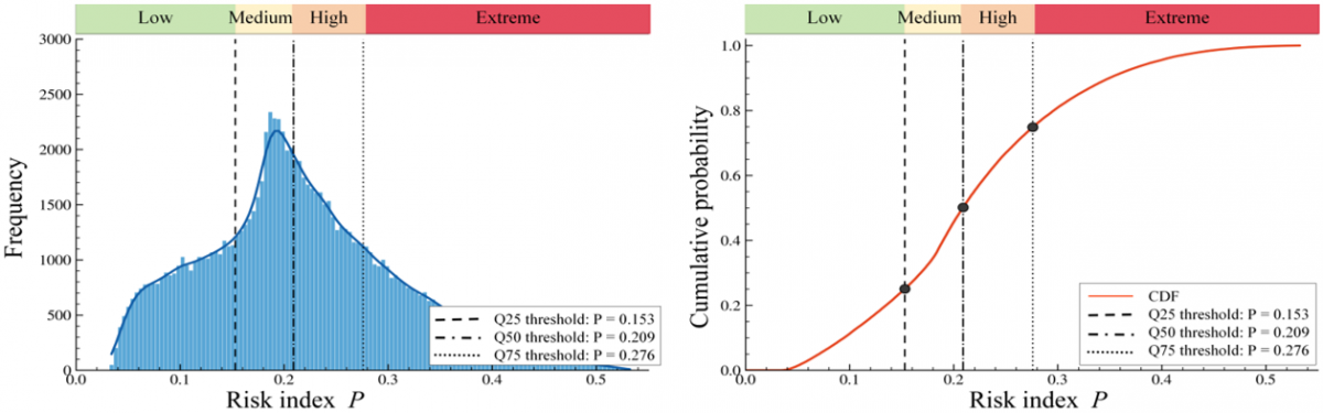
Specifically, RA, RD, and RV are assumed to follow independent uniform distributions over the interval [0.2, 1.0]. The model undergoes (N = 100,000) random sampling simulations. Each simulation yields a triplet (V, A, D), which is then substituted into the Target Loss Probability Model in Eq. (2) to calculate the corresponding Target Loss Probability index P. The simulation results are shown in Figure 1. The results indicate that the Target Loss Probability index is distributed within [0.0312, 0.5318]. With reference to the quartiles of the simulated data, this study divides the Target Loss Probability index into four relative risk levels: Low, Medium, High, and Extreme. The corresponding thresholds are shown in Table 4.
Figure 1. Distribution and cumulative distribution of Target Loss Probability index
To examine whether the risk-grading thresholds are sensitive to the assumed input distribution, this study further conducts a distributional robustness check at the model-construction stage. In addition to the baseline uniform distribution, two alternative distributions are considered. The first is a triangular distribution with lower bound 0.2, mode 0.6, and upper bound 1.0. The mode 0.6 is the midpoint of the standardized interval and represents a neutral medium-level assumption. The second is a scaled beta distribution 0.2 + 0.8 × Beta (2, 2), which also concentrates more probability mass around the middle of the standardized interval. These two distributions are used to test whether the quartile-based risk thresholds remain relatively stable when the input parameters are no longer uniformly distributed. The robustness check results under the three input distribution assumptions are summarized in Table 5. The robustness results show that the quartile thresholds vary only within a limited range under different input distribution assumptions. The Q50 threshold remains around 0.21–0.23, and the Q75 threshold remains around 0.27. This indicates that the Monte Carlo-based risk grading matrix is not highly sensitive to the baseline uniform distribution assumption. Therefore, the thresholds obtained in this section can be used as relative internal grading criteria for subsequent case analysis under the proposed model.
Table 4. Relative risk grading thresholds for the Target Loss Probability index
|
Lower Bound of Risk Index Interval |
Upper Bound of Risk Index Interval |
Risk Level |
|
0.0312 |
0.153 |
Low |
|
0.153 |
0.209 |
Medium |
|
0.209 |
0.276 |
High |
|
0.276 |
0.532 |
Extreme |
Table 5. Robustness check of Monte Carlo-based risk grading thresholds under different input distributions
|
Distribution |
Q25 |
Q50 |
Q75 |
Interpretation |
|
Uniform U (0.2, 1.0) |
0.153 |
0.209 |
0.276 |
Baseline non-informative assumption |
|
Triangular Tri (0.2, 0.6, 1.0) |
0.189 |
0.226 |
0.268 |
Medium-centered distribution |
|
Scaled beta 0.2 + 0.8 × Beta (2, 2) |
0.178 |
0.222 |
0.271 |
Medium-concentrated distribution |
To verify the calculation process and application value of the proposed framework, this study constructs an anonymized coastal nuclear-facility scenario for case analysis. Considering the sensitivity of security information related to critical infrastructure and key assets, this study does not disclose the facility name, exact geographical location, actual equipment deployment, specific detection blind spots, emergency response records, or other security-sensitive details. The scenario is not intended to evaluate the actual security status of a specific real facility, but to demonstrate how the proposed Target Loss Probability Model can be applied under data-scarce and security-sensitive conditions.
The non-sensitive assumptions of the scenario are as follows. First, the target is assumed to be a coastal nuclear facility with high strategic value, strong public-safety relevance, and potentially severe social consequences if disrupted. Second, the threat scenario assumes low-altitude UAS intrusion risks, including reconnaissance, disruption, and possible physical intrusion toward key protected areas. Third, the existing defensive system is assumed to include detection, identification, countermeasure, physical-barrier, and security-management capabilities, but the performance of these capabilities may be affected by coastal environmental complexity, low-altitude approach routes, and small-target detection difficulty. Fourth, the expert scoring is based on publicly available knowledge of nuclear-facility protection, general C-UAS system characteristics, and the five-level scoring rubrics provided in Supplementary Material A, rather than on confidential facility-specific data.
3.1 Application of the Target Loss Probability Model for unmanned aircraft system threat risk assessment
To improve the reliability and transparency of expert judgment, this study established explicit criteria for expert selection. Ten experts were invited to participate in the indicator scoring process. The experts were selected according to the following criteria: (1) having at least five years of professional or research experience in risk assessment, critical infrastructure protection, nuclear-facility safety/security, security protection, or counter-UAS-related fields; (2) holding senior professional qualifications or having recognized senior-level industry experience in the relevant field; (3) being familiar with risk assessment framework construction, indicator screening, and indicator weighting; and (4) being willing to participate in multiple rounds of questionnaire scoring and to ensure the completeness of their responses.
To protect personal privacy and security-sensitive information, the names and institutional affiliations of the experts are not disclosed. Instead, the experts are coded as E1-E10. The background information of the expert panel is summarized in Table 6.
Table 6. Background information of the expert panel
|
Expert Code |
Expertise Field |
Years of Experience |
Senior Qualification/Professional Background |
|
E1 |
Security protection |
≥10 years |
Senior practitioner |
|
E2 |
Security protection |
5–10 years |
Senior professional qualification |
|
E3 |
Critical infrastructure protection |
≥10 years |
Senior practitioner |
|
E4 |
Nuclear-facility safety/security |
≥10 years |
Senior professional background |
|
E5 |
Nuclear-facility safety/security |
5–10 years |
Senior practitioner |
|
E6 |
Counter-unmanned aircraft system (UAS) technology |
≥10 years |
Senior technical expert |
|
E7 |
Counter-UAS technology |
5–10 years |
Senior practitioner |
|
E8 |
Risk assessment |
≥10 years |
Senior researcher |
|
E9 |
Emergency/Security management |
5–10 years |
Senior practitioner |
|
E10 |
Low-altitude security/UAS risk |
5–10 years |
Senior practitioner |
To further examine the reliability of expert scoring, Kendall’s coefficient of concordance was used to test the consistency of expert judgments. The consistency test was conducted separately for the attacker-resource, defensive-resource, and target-value subsystems. The Kendall’s W values for the three subsystems were 0.7948, 0.9538, and 0.9000, respectively, and all passed the chi-square significance test (p < 0.001), indicating statistically significant and acceptable consistency among expert judgments. The relatively high consistency may be attributed to the use of unified five-level scoring rubrics, clearly defined indicator meanings, and the similar professional backgrounds of the expert panel. Therefore, the expert scoring results were considered suitable for subsequent weighting and model calculation.
The mean expert scores were combined with the final combined weights obtained by the Maximizing Deviation Method to calculate the subsystem indices. Specifically, the weighted score of each level-3 indicator was obtained by multiplying its mean expert score by the corresponding combined weight, and the subsystem index was obtained by summing all weighted scores within the corresponding subsystem. The complete weights and weighted calculation results for RA, RD, and RV are provided in Supplementary Material B. According to these weighted calculation results, the three model inputs for the anonymized nuclear-facility scenario are obtained as V = 0.8722, A = 0.7615, and D = 0.5542. Substituting these values into the Target Loss Probability Model yields a Target Loss Probability index of p = 0.2542. Referring to Table 4, the UAS threat risk in this scenario is classified as “High”.
With RV and RA held constant, this study further calculates the model-recommended defensive resource capability level. Previous studies applying the Target Loss Probability Model to security prevention system evaluation have shown that, after the RV, RA, and RD are determined, the model can be used not only to calculate the Target Loss Probability, but also to derive a model-recommended defensive resource value for guiding subsequent resource improvement. Following this logic, the defensive resource capability value calculated in this study should be interpreted as a model-recommended target level rather than an empirically observed value. Specifically, based on the Target Loss Probability Model, Eqs. (7) and (8) are used to calculate the model-recommended defensive resource capability value under the given RV and RA conditions [18]. Substituting (V = 0.8722) and (A = 0.7615) into the model yields a recommended defensive resource capability value of ($D^0$ = 0.8245).
$\begin{array}{r}A^0(V, D)=\frac{V^{\frac{3}{2}}}{D}+\frac{1}{9} \sqrt{V^3+27 \sqrt{3} \frac{V^3}{D^2}}-\frac{1}{3} \times \frac{V}{\frac{V^{\frac{3}{2}}}{D}+\frac{1}{9} \sqrt{V^3+27 \sqrt{3} \frac{V^3}{D^2}}}\end{array}$ (7)
$D^0=\frac{\sqrt{V}}{A^0} \times \ln \left|\frac{V}{E L} \times \frac{\left(A^0\right)^2}{\left(A^0\right)^2+V}\right|$ (8)
We assume that RA and RV remain constant. Substituting the model-recommended RD $D^0$ into the model yields a new Target Loss Probability $P^0$ of 0.2039. The risk level downgrades from "High" to "Medium." The defensive resource capability index increases by approximately 48.77%. The Target Loss Probability index can be reduced by 19.79%. These results are presented in Table 7.
Table 7. Comparison between current and improved defensive resource states
|
State |
|
|
|
|
Risk Level |
|
Current state |
0.8722 |
0.7615 |
0.5542 |
0.2542 |
High |
|
Improved state |
0.8722 |
0.7615 |
0.8245 |
0.2039 |
Medium |
|
Change magnitude |
|
|
+48.77% |
-19.79% |
Downgraded one level |
3.2 Defensive resource sensitivity prioritization based on Sobol analysis
The ultimate goal of risk assessment lies in reducing Target Loss Probability through rational prioritization of defensive resource improvement. However, RD comprises 18 Level-3 indicators. Comprehensive upgrading would be both costly and inefficient. To identify key weaknesses and leverage points in the defense system, this study employs Sobol global sensitivity analysis [19]. This quantifies the contribution of uncertainty in each Level-3 indicator of $\text{D}$ to the variance of Target Loss Probability $\text{P}$. We thereby screen out key indicators most sensitive to risk reduction and guide defensive resource improvement.
3.2.1 Sobol model construction and parameter setting
The Sobol method decomposes model output variance into contributions from individual input variables and their interactions. For the UAS threat risk assessment model in this study, we construct the analysis framework as follows:
Eq. (2) from the Target Loss Probability Model serves as the response function for sensitivity analysis $Y=f(V, A, D)$:
$Y=f(V, A, D)=\exp \left(-\frac{A \cdot D}{\sqrt{V}}\right) \times \frac{A^2}{A^2+V}$ (9)
RD D are aggregated from its 18 tertiary indicators through weighted summation:
$D=\sum_{i=1}^{i=18} \omega_i^{(D)} \cdot R D_i$ (10)
where, $\omega_i{ }^{(D)}$ represents the combined weight of each indicator for RD D. These weights are determined via the Maximizing Deviation Method in Section 2.3. RA is fixed at A = 0.7615, and RV is fixed at V = 0.8722. Sobol analysis is performed on the 18 tertiary indicators of D. To comprehensively examine the impact of each indicator on risk, all defender resource indicators are set to follow a uniform distribution: $X_{R D_i} \sim U(0.2,1.0)$. The Saltelli sampling sequence is employed to generate the input sample matrix. The base sample size is set to N = 1024. The input variable dimension is k = 18. Using Saltelli sampling, the total number of model runs is N (2k + 2). This ensures the convergence and accuracy of both the firstorder sensitivity index $\left(S_1\right)$ and the total-effect sensitivity index $\left(S_T\right)$.
3.2.2 Sobol index calculation and results
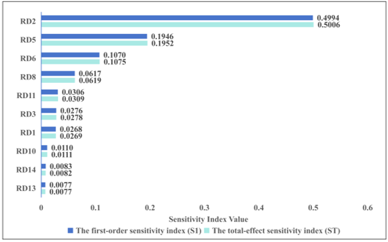
Python is used to implement Monte Carlo sampling and model computation. The sensitivity indices of each defense indicator are then output. Simulation results are shown in Figure 2.
As shown in Figure 2, the total-effect index of detection coverage rate $\mathrm{RD}_2$ reaches 0.5006. This accounts for half of the single-indicator contribution. Detection accuracy $\mathrm{RD}_5$ and identification accuracy $\mathrm{RD}_6$ rank second and third, respectively. Their cumulative contribution exceeds 80%. Considering the complex coastal environment in the case scenario and the difficulty of detecting low-altitude targets, these results indicate that the main weakness of the current system lies in insufficient detection capability. From the perspective of defensive resource prioritization, the performance bottleneck of the defense system is mainly concentrated in the front-end perception chain. Identification response time $\mathrm{RD}_8$ and countermeasure engagement range $\mathrm{RD}_{11}$ also rank in the top five. However, their sensitivity indices fall below 0.07. This indicates relatively weak marginal improvement effects on risk. These findings demonstrate that enhancing front-end detection capability reduces risk more effectively than simply increasing countermeasure weapons.
Figure 2 shows that $S_1$ and $S_T$ are highly similar for each indicator. This suggests weak nonlinear coupling among defense elements under the current indicator system. These elements mainly influence risk values through independent effects. Consequently, security managers can prioritize independent upgrades for single vulnerabilities. This suggests that targeted improvement of individual key indicators is feasible without requiring major system-wide restructuring.
Figure 2. Sobol sensitivity indices of top 10 defensive resource indicators
3.2.3 Sensitivity-based defensive resource prioritization and verification
Based on the analysis of simulation results in Section 3.2.2, this section presents the defensive resource prioritization strategy. Details are shown in Table 8.
It should be noted that the measures listed in Table 8 should be interpreted as sensitivity-based technical prioritization results rather than a complete cost-minimization or investment-optimization plan. The Sobol sensitivity results identify the defensive indicators that have greater influence on the Target Loss Probability index, but actual implementation still needs to consider budget constraints, procurement cycles, site conditions, system compatibility, maintenance requirements, operator training, electromagnetic compatibility, and regulatory authorization.
From an implementation perspective, improving detection coverage rate and detection accuracy should be regarded as first-stage technical priorities because they show the highest sensitivity contributions and directly affect the front-end perception capability of the defensive system. Improvements in identification accuracy and identification response time can be implemented as medium-priority measures because they are more likely to rely on software upgrading, workflow optimization, feature-database construction, and personnel training. By contrast, extending the countermeasure engagement range may involve higher equipment costs, regulatory constraints, and operational restrictions, and should therefore be implemented cautiously according to site-specific conditions and compliance requirements. Therefore, the measures in Table 8 provide decision support for identifying high-impact defensive weaknesses, while the final implementation plan should be determined by facility managers according to available budget, operational feasibility, maintenance capacity, and regulatory compliance. Similar data availability and methodological transferability challenges have also been noted in critical-infrastructure risk-assessment research [20].
Based on the prioritization strategy in Table 8, other indicators remain at their current scores. The improved $D^*$ is calculated as approximately 0.831 using Eq. (10). This value is highly consistent with the $D^0$(0.8245) obtained in Section 3.1. Substituting $D^*$ into the Target Loss Probability Model yields a new Target Loss Probability $P^*$ of 0.2028. The risk level is successfully downgraded from “High” to “Medium”.
Table 8. Sensitivity-based defensive resource prioritization and improvement measures
|
Key Indicator |
Current Score |
Suggested Improvement Measure |
Improved Score |
|
Detection Coverage Rate $\mathrm{RD}_2$ |
0.6 |
Deploy passive detection equipment and integrate radar, RF, and electro-optical sensing for multi-source fusion detection. |
1.0 |
|
Detection Accuracy $\mathrm{RD}_5$ |
0.4 |
Introduce spectrum detection equipment and upgrade radar signal-processing algorithms to reduce false alarms. |
0.8 |
|
Identification Accuracy $\mathrm{RD}_6$ |
0.6 |
Install AI-enabled electro-optical identification modules and establish a localized low-slow-small unmanned aircraft system (UAS) feature database. |
0.8 |
|
Identification Response Time $\mathrm{RD}_8$ |
0.6 |
Upgrade the command platform to support automated alarm, identification, and response workflows. |
0.8 |
|
Countermeasure Engagement Range $\mathrm{RD}_{11}$ |
0.4 |
Configure long-range GNSS spoofing equipment and improve frequency-band coverage and engagement range. |
0.8 |
This study proposes a risk assessment and defensive prioritization method based on the Target Loss Probability Model for UAS threats against critical infrastructure and key assets. Through the construction of a three-dimensional indicator system incorporating RV, RA, and RD, and through a combined weighting strategy based on the Maximizing Deviation Method, this study addresses the weighting problem under small-sample data conditions. In addition, Monte Carlo simulation is used to establish relative grading thresholds for the nonlinear model output. This study introduces Sobol global sensitivity analysis. It reveals that detection coverage rate and detection accuracy are the first-order dominant factors of system risk. The anonymized nuclear facility case study demonstrates that the proposed method can transform qualitative UAS threat factors into a structured and computable risk assessment process. Increasing the defensive resource capability index by 48.77% reduces the Target Loss Probability index by 19.79%. This results in a one-level reduction in the relative risk level from “High” to “Medium”. The method provides auxiliary decision support for prioritizing counter-UAS defensive resource improvement for critical infrastructure and key assets.
Nevertheless, the case study is based on an anonymized scenario and small-sample expert scoring, which may limit the direct generalization of the numerical results. Future research may further validate the proposed framework using multi-scenario datasets, larger expert panels, and dynamic UAS attack-defense simulations.
This work is supported by the Top Innovative Talent Training Program of People’s Public Security University of China (Grant No.: 2026yjskcjs041).
|
A |
Attacker resource capability index, dimensionless |
|
D |
Defensive resource capability index, dimensionless |
|
|
|
|
EL |
Expected loss, dimensionless |
|
N |
Number of Monte Carlo simulations |
|
p |
Target Loss Probability index, dimensionless |
|
RA |
Attacker-resource indicator code, dimensionless |
|
RD |
Defensive-resource indicator code, dimensionless |
|
RV |
Target-Value indicator code, dimensionless |
|
S1 |
First-order Sobol sensitivity index, dimensionless |
|
ST |
Total-effect Sobol sensitivity index, dimensionless |
|
V |
Target value index, dimensionless |
|
w |
Indicator weight, dimensionless |
|
x |
Indicator score, dimensionless |
|
i |
Index of target or indicator |
|
j |
Index of indicator |
[1] Chamola, V., Kotesh, P., Agarwal, A., Naren, Gupta, N., Guizani, M. (2021). A comprehensive review of unmanned aerial vehicle attacks and neutralization techniques. Ad Hoc Networks, 111: 102324. https://doi.org/10.1016/j.adhoc.2020.102324
[2] Kunertova, D. (2023). Drones have boots: Learning from Russia’s war in Ukraine. Contemporary Security Policy, 44(4): 576-591. https://doi.org/10.1080/13523260.2023.2262792
[3] International Energy Agency. (2024). Ukraine’s Energy Security and the Coming Winter. International Energy Agency. https://www.iea.org/reports/ukraines-energy-security-and-the-coming-winter/ukraines-energy-system-under-attack.
[4] European Union. (2022). Directive (EU) 2022/2557 of the European Parliament and of the Council of 14 December 2022 on the resilience of critical entities and repealing Council Directive 2008/114/EC. Official Journal of the European Union, OJ L 333: 164-198. http://data.europa.eu/eli/dir/2022/2557/oj.
[5] European Union Aviation Safety Agency (EASA). (2020). Opinion No. 01/2020: High-level regulatory framework for the U-space. Cologne: European Union Aviation Safety Agency. https://www.easa.europa.eu/en/document-library/opinions/opinion-012020.
[6] Yang, Z., Barroca, B., Laffréchine, K., Weppe, A., Bony-Dandrieux, A., Daclin, N. (2023). A multi-criteria framework for critical infrastructure systems resilience. International Journal of Critical Infrastructure Protection, 42: 100616. https://doi.org/10.1016/j.ijcip.2023.100616
[7] Schotten, R., Mühlhofer, E., Chatzistefanou, G.A., Bachmann, D., Chen, A.S., Koks, E.E. (2024). Data for critical infrastructure network modelling of natural hazard impacts: Needs and influence on model characteristics. Resilient Cities and Structures, 3(1): 55-65. https://doi.org/10.1016/j.rcns.2024.01.002
[8] Major, A.J. (2002). Advanced techniques for modeling terrorism risk. The Journal of Risk Finance, 4(1): 15-24. https://doi.org/10.1108/eb022950
[9] Garcia, M.L. (2005). Vulnerability Assessment of Physical Protection Systems. Oxford: Elsevier Butterworth-Heinemann.
[10] Likert, R. (1932). A technique for the measurement of attitudes. Archives of Psychology, 140: 1-55. https://psycnet.apa.org/record/1933-01885-001.
[11] European Union. (2019). Commission implementing regulation (EU) 2019/947 of 24 May 2019 on the rules and procedures for the operation of unmanned aircraft. Official Journal of the European Union, L152: 45-71. http://data.europa.eu/eli/reg_impl/2019/947/oj.
[12] Joint Air Power Competence Centre (JAPCC). (2021). A Comprehensive Approach to Countering Unmanned Aircraft Systems. NATO JAPCC, Kalkar. https://www.japcc.org/books/a-comprehensive-approach-to-countering-unmanned-aircraft-systems.
[13] ISO. (2018). ISO 31000:2018 Risk management — Guidelines. International Organization for Standardization, Geneva. https://www.iso.org/standard/65694.html.
[14] European Union Aviation Safety Agency (EASA). (2023). EASA Artificial Intelligence Roadmap 2.0: A human-centric approach to AI in aviation. Cologne: European Union Aviation Safety Agency. https://www.easa.europa.eu/en/document-library/general-publications/easa-artificial-intelligence-roadmap-20.
[15] Wang, J., Liu, Y., Song, H. (2021). Counter-Unmanned Aircraft System(s) (C-UAS): State of the art, challenges, and future trends. IEEE Aerospace and Electronic Systems Magazine, 36(3): 4-29. https://doi.org/10.1109/MAES.2020.3015537
[16] Li, X., Wang, K., Liu, L., Xin, J., Yang, H., Gao, C. (2011). Application of the entropy weight and TOPSIS method in safety evaluation of coal mines. Procedia Engineering, 26: 2085-2091. https://doi.org/10.1016/j.proeng.2011.11.2410
[17] Arunraj, N.S., Mandal, S., Maiti, J. (2013). Modeling uncertainty in risk assessment: An integrated approach with fuzzy set theory and Monte Carlo simulation. Accident Analysis & Prevention, 55: 242-255. https://doi.org/10.1016/j.aap.2013.03.007
[18] Si, G., Chen, W., Hu, X., Zhang, P. (2025). Efficiency evaluation on security and prevention systems of bank vaults based on Target Loss Probability model. Journal of University of Jinan (Science and Technology), 719-726. https://doi.org/10.13349/j.cnki.jdxbn.20241225.001
[19] Puy, A., Becker, W., Lo Piano, S., Saltelli, A. (2022). A comprehensive comparison of total-order estimators for global sensitivity analysis. International Journal for Uncertainty Quantification, 12(2): 1-18. https://doi.org/10.1615/Int.J.UncertaintyQuantification.2021038133
[20] Pasino, A., De Angeli, S., Battista, U., Ottonello, D., Clematis, A. (2021). A review of single and multi-hazard risk assessment approaches for critical infrastructures protection. International Journal of Safety and Security Engineering, 11(4): 305-318. https://doi.org/10.18280/ijsse.110403