Yamama A. Shafeek* | Mohammed Majid Msallam | Huthaifa Al-Khazraji
© 2026 The authors. This article is published by IIETA and is licensed under the CC BY 4.0 license (http://creativecommons.org/licenses/by/4.0/).
OPEN ACCESS
Energy consumption is a key competitive factor in manufacturing, as accurate prediction directly supports production optimization. Therefore, manufacturers increasingly focus on improving energy efficiency to remain competitive. This paper develops a novel framework for estimating energy consumption of steel production. The proposed framework employs two prediction models: the first uses the full preprocessed dataset, while the second uses a SHapley Additive exPlanation (SHAP)-refined dataset with selected features removed. The explainability-driven refinement aims to improve prediction performance and model robustness. After the dataset has been processed and normalized, the deep neural network (DNN) model is used for the prediction. The proposed DNN model is used to develop the prediction model. It consists of one input and one output layer, plus three hidden layers. All five layers are arranged as stacked layers sequentially. Computer simulation results reveal that the proposed DNN approach achieves a superior prediction rate. The Root Mean Squared Error (RMSE) value for the testing results is reduced from 1.97 in the case of Support Vector Machine (SVM), 2.99 in the case of K Nearest Neighbor (KNN) and 1.12 in the case of Random Forest (RF) to 0.31 in the proposed DNN model. These findings imply that the proposed DNN model is more capable of the energy consumption's prediction.
electric systems, artificial intelligence, deep neural network, energy consumption, prediction model
Energy consumption is a primary consideration in the development of global manufacturing industries. It can have various forms such as electricity, gas, and diesel [1, 2]. Studies show that the industrial sector leads all other sectors of global energy consumption. As of 2021, industry domain consumed 33% of the total energy in the United States [3]. Energy waste and over-consumption are the main causes of this high level of consumed energy [4, 5]. Thus, prediction is considered an essential tool in most industrial companies. Having an estimation of the expected usage of energy, makes it possible to decide the level of operation that is to be expected. Therefore, implementing energy prediction and developing an efficient management of energy has the benefit of reducing energy consumption.
With the availability of data, Artificial Intelligence (AI) can be used to investigate and explore the energy consumption patterns. In recent years, AI has exhibited outstanding performance for solving many problems. It has been used as a tool for decision-making processes and successfully applied for many industrial applications [6-10]. In addition, the availability of data collected from various sources has become one of the pillars of modern manufacturing [5]. During seeking improvement of accuracy of prediction models, various AI-based prediction models have been proposed. For instance, Sathishkumar et al. [11] evaluated five models, namely: General Linear Regression (GLR), Support Vector Machine (SVM) with Radial Basis Kernel, Classification and Regression Trees (CRT), K Nearest Neighbor (KNN), and Random Forest (RF), using real data for the steel industry. For the purpose of evaluation, four indices were used. The results showed that the RF model has lower Root Mean Squared Error (RMSE), Mean Absolute Error (MAE), Mean Absolute Percentage Error (MAPE), and Coefficient of Variation (CV) values than other prediction models.
Afzal et al. [12] proposed energy predictive models using a multilayer perceptron neural network (MLP). Eight meta-heuristic algorithms were employed to fine-tune the hyperparameters of the MLP model. The results revealed that the MLP-PSOGWO model method has the most promising result with better accuracy. Mahjoub et al. [13] compared three different algorithms for power consumption forecasting. Real data of power consumption in some French cities were used to evaluate these methods. The outcomes revealed that the long short-term memory model yields a better outcome than the gated recurrent unit and the Drop-GRU methods. On the other hand, Dinmohammadi et al. [14] utilized the practical swarm optimization (PSO) to enhance the FR prediction model's performance for residential heating energy consumption. The optimization technique was used to select the features, while the RF was used for performance evaluation of their subsets. The proposed model showed superior performance compared with other models such as the KNN, eXtreme Gradient Boosting (XGBoost), and CatBoost. Pham et al. [15] presented another prediction model based on RF to estimate the usage of energy in multiple buildings. The hourly building energy consumption dataset for five years was adapted to test the efficacy of the RF model. The results revealed that the RF model was outperformed by the Random Tree (RT) models.
In building a deep neural network (DNN), a basic neural network is extended by introducing two or more hidden layers. The DNN model is an effective tool for learning complex patterns with high-dimensional datasets. Therefore, it has been used as a sportive tool for many industrial applications such as forecasting of energy consumption [16], defect detection [17, 18], and evaluation of system reliability [19]. The use of DNNs provides a dual advantage: they not only streamline model deployment but also enhance prediction accuracy. In this context, this paper proposes a novel DNN model that is structured with a total of five layers (one input layer, followed by three hidden layers, then by one output layer). All five layers were arranged as stacked layers sequentially. A comparison between the proposed prediction DNN model and the SVM, KNN, and RF has been conducted using published consumption energy data of the steel industry. Moreover, for the purpose of identifying the most important features of the used dataset, in this work, the SHapley Additive exPlanation (SHAP) is used [20, 21]. For this purpose, two models based on DNN will be developed. One is based on the dataset, whereas the other is based on the importance feature that is obtained by SHAP. Thus, the contribution of this study can be stated as follows: 1) Examine the effectiveness of DNN models in predicting industrial energy consumption patterns. 2) Utilize SHAP method to extract the important features for a given dataset by underlying relationships between features and the outcome. 3) Deliver an effective solution to support high-level industrial managers in getting a clear apprehension of energy performance and thereby enhancing production energy efficiency.
The paper is prepared as follows. Section 2 presents the methodology of the work regarding the proposed DNN prediction model, data processing, and the evaluation indices. The simulation experiment study and comparisons with other prediction models are presented in Section 3. Finally, a summary of the paper is given in Section 4.
The methodology consists of three pillars. The first one provides the details of the proposed artificial neural network (ANN) architecture model. The second describes the dataset, which was obtained from DAEWOO Steel Company in Gwangyang city, South Korea. Eliminating redundant data was performed before processing the data. The last pillar gives the evaluation indices that were employed to evaluate the proposed prediction model.
2.1 Proposed model
ANN has the advantage of learning complex dynamics. It is widely used for classification, predictions, and pattern recognition. The general architecture of the ANN consists of layers, neurons, and weights that connect the neurons [22-24]. DNN is a sort of ANN that is subsequently developed based on machine learning (ML) [25, 26]. Its model is formed by multiple layers, which are composed of artificial neurons. Every layer in the DNN learns a different level of abstraction from the training data [27, 28]. These layers learn to distinguish differences based on the huge dataset. The learned layers and links between them give the trained model of the DNN. The links between layers are called architecture model [29]. The architecture model is pivotal to the accuracy of the estimation and the complexity and simplification of the model. Algorithm 1 below illustrates the Pseudo-code of a generalized DNN.
|
Algorithm 1. Pseudo-code of generalized Deep Neural Network |
|
1. Initialize network parameters: - For each layer: - Initialize weights W[l] with random values 2. Repeat until convergence (e.g., until loss is below a threshold or max epochs reached): For each training example: a. Forward Pass: - Set activation A[0] = x - For each layer l in 1 to L: - $Z[l]=W[l] * A[l-1]$ - A[l] = activation_function(Z[l]) b. Compute Loss: - loss = loss_function(A[L], y) c. Backpropagation: - Compute derivative of loss w.r.t. output activation: dA[L] = derivative_loss(A[L], y) - For each layer l from L down to 1: - dZ[l] = dA[l] * derivative_activation(Z[l]) - dW[l] = dZ[l] * A[l-1]^T - db[l] = dZ[l] - dA[l-1] = W[l]^T * dZ[l] d. Update Parameters: - For each layer l in 1 to L: - W[l] = W[l] - learning_rate * dW[l] - b[l] = b[l] - learning_rate * db[l] |
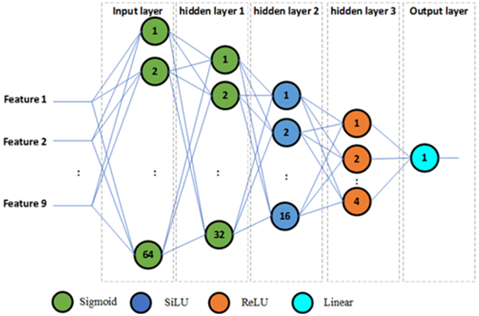
The designed model in this work is shown in Figure 1. As depicted, all five layers are arranged as stacked layers sequentially, with lots of artificial neurons in the top layer and fewer artificial neurons in the end.
Figure 1. Proposed deep neural network (DNN) architecture model
The activation functions used in each layer and the input/output sizes of each layer of the proposed model are listed in Table 1. The proposed DL model uses four activation functions: sigmoid, Sigmoid Linear Unit (SiLU), Rectified Linear Unit (ReLU), and linear activation functions. The sigmoid activation function restrains a real number to a value between 0 and a positive constant, as in the mathematical expression in Eq. (1).
$f(x)=\frac{1}{1+e^{-a x}}$ (1)
Table 1. The details of layers
|
Layer |
Activation Function |
Input Size |
Output Size |
|
Input layer |
Sigmoid |
(None, 9) |
(None, 64) |
|
Hidden layer_1 |
Sigmoid |
(None, 64) |
(None, 32) |
|
Hidden layer_2 |
SiLU |
(None, 32) |
(None, 16) |
|
Hidden layer_3 |
ReLU |
(None, 16) |
(None, 4) |
|
Output layer |
Linear |
(None, 4) |
(None, 1) |
On the other hand, SiLU multiplies the input by the result of the sigmoid activation function; its mathematical equation is expressed by:
$f(x)=\frac{x}{1+e^{-b x}}$ (2)
Alternatively, the ReLU function sets all negative values in the input to zero and keeps all positive values as in the mathematical expression in Eq. (3).
$f(x)=\max (0, x)$ (3)
Finally, the linear activation function results in a directly proportional value to the input, as in the mathematical expression in Eq. (4) [9, 30, 31].
$f(x)=c x$ (4)
where, a, b and c are constant values. These constants affect the accuracy of the model and its learning, and due to be careful in choosing their values. Based on our experience in building models, the appropriate values a, b, and c are 1, 3 and 2, respectively.
2.2 Processing dataset
The dataset was obtained from DAEWOO, a steel manufacturing company based in South Korea. The company utilizes a cloud-based system to store its data, which includes daily, monthly, and yearly energy consumption records. This information is publicly accessible via the website (pccs.kepco.go.kr) [11]. The dataset is presented in Table 2. It has eleven features with 35040 samples for each feature. The eight features are continuous values, while the three are categorical values. The categorical features are week status, day of week and load type, which contain two, seven and three categories, respectively. The dataset will be processed before training the model. At first, the dataset will be read by the pandas library using Python.
Table 2. Dataset description
|
Name of Data |
Classification |
Unit |
|
Date |
Continuous |
Time |
|
Energy Consumption |
Continuous |
kWh |
|
Leading Current Reactive Power |
Continuous |
kVarh |
|
Lagging Current Reactive Power |
Continuous |
kVarh |
|
Leading Current Power Factor |
Continuous |
% |
|
Lagging Current Power Factor |
Continuous |
% |
|
tCO2(CO2) |
Continuous |
ppm |
|
Number of Seconds from Midnight |
Continuous |
second |
|
Week Status |
Categorical |
(Weekend (0) or a Weekday (1)) |
|
Day of Week |
Categorical |
Sunday, Monday …. Saturday |
Table 3. Dataset before and after processing
|
Feature |
Data Type |
Sample 1 |
Sample 2 |
Sample 3 |
|
Energy Consumption |
Raw dataset |
3.96 |
51.26 |
54.79 |
|
Processed dataset |
3.96 |
51.26 |
54.79 |
|
|
Lagging Current Reactive Power |
Raw dataset |
4.68 |
4.54 |
7.52 |
|
Processed dataset |
0.507 |
0.516 |
0.332 |
|
|
Leading Current Reactive Power |
Raw dataset |
0 |
0.94 |
0.14 |
|
Processed dataset |
0.524 |
0.397 |
0.505 |
|
|
tCO2(CO2) |
Raw dataset |
0 |
0 |
0 |
|
Processed dataset |
0.709 |
0.709 |
0.709 |
|
|
Lagging Current Power Factor |
Raw dataset |
64.59 |
99.61 |
99.07 |
|
Processed dataset |
0.84 |
-0.10 |
-0.976 |
|
|
Leading Current Power Factor |
Raw dataset |
100 |
99.98 |
100 |
|
Processed dataset |
-0.515 |
-0.514 |
-0.515 |
|
|
NSM |
Raw dataset |
17100 |
34200 |
36900 |
|
Processed dataset |
1.03 |
0.34 |
0.231 |
|
|
Week Status |
Raw dataset |
Weekday |
Weekday |
Weekday |
|
Processed dataset |
0 |
0 |
0 |
|
|
Day of Week |
Raw dataset |
Tuesday |
Tuesday |
Tuesday |
|
Processed dataset |
0.1428 |
0.1428 |
0.1428 |
|
|
Load Type |
Raw dataset |
Light_Load |
Medium_Load |
Maximum_Load |
|
Processed dataset |
0 |
0.333 |
0.666 |
Normalization is applied to all continuous features in the dataset by standardizing each feature, whereby the mean value was subtracted and the result was divided by the corresponding standard deviation. For categorical features, categorical encoding was performed by assigning a numerical representation to each category based on the total number of categories associated with that feature.
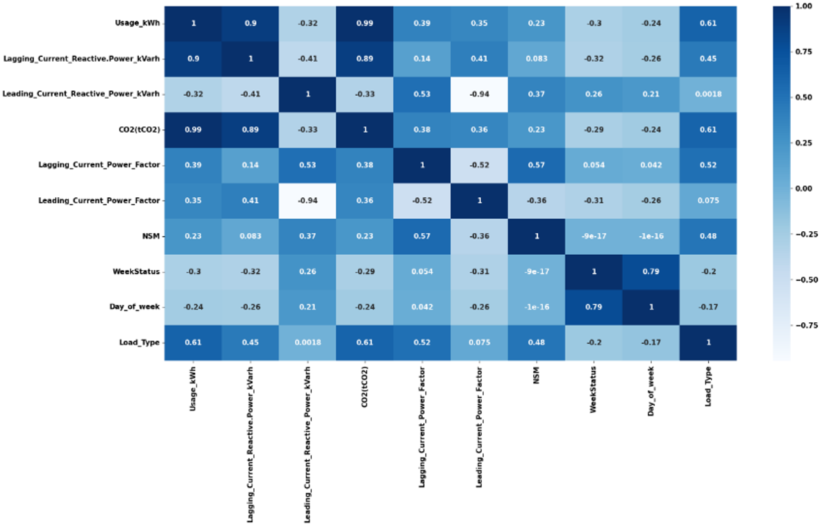
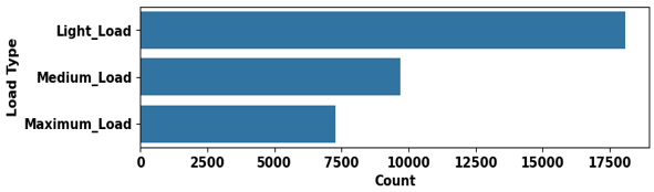
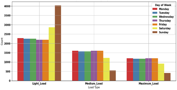
An example illustrating the raw and preprocessed datasets is provided in Table 3. The features in the dataset exhibit weak intercorrelations, suggesting a low degree of redundancy among them. Consequently, each feature contributes unique and complementary information to the analysis, enhancing the model's ability to capture diverse patterns within the data. This diversity of information can improve the learning process and promote better generalization performance. The highest correlation between the CO2(tCO2) feature and the Usage_kWh feature is 0.61, as shown in Figure 2. The work of the company is classified into three categories (light load, medium load, and maximum load). Most of the recorded samples were light, while the recorded samples of maximum load were the fewest, as shown in Figure 3. These categories by day of the week are distributed between weekdays and weekends, as shown in Figure 4. Weekdays consistently exhibit high and similar counts for medium load and maximum load, indicating generally demanding load conditions.
Figure 2. The correlation matrix of the dataset features
Figure 3. Load type
Figure 4. Load type distribution by day of week
In contrast, light load is most prevalent on Sundays, which also shows the lowest occurrences of medium load and maximum load, suggesting Sundays are the least demanding in terms of load. Saturdays typically present a reduction in medium and maximum loads compared to weekdays, but not as drastically as Sundays, while still maintaining a significant level of light Load that is less dominant than on Sundays. Conversely, the maximum energy consumption of the company is 157.18 kWh.
2.3 Evaluation indices
To evaluate the proposed DNN prediction model and to capture the goodness of fit and deviation of the prediction data from the real data, RMSE as given in Eq. (5), MAE as given in Eq. (6), and CV as given in Eq. (7) indices are used [8, 32-34].
$R M S E=\sqrt{\frac{\sum_{i=0}^n\left(A_i-F_i\right)^2}{n}}$ (5)
$M A E=\frac{1}{n} \sum_{i=0}^n\left|A_i-F_i\right|$ (6)
$C V=\frac{R M S E}{\hat{Y}_{{data}}} \times 100$ (7)
where, i, n, A, F and $\widehat{\mathrm{Y}}_{\text {data}}$ are the index for the data, the size of the data, the actual data, the estimated data, and the average energy consumption.
The proposed DNN model is implemented on a personal computer (PC) with an AMD Ryzen 7 processor, eight gigabytes of Random Access Memory (RAM), and eight gigabytes of video memory. The 64-bit Windows 11 Home operating system is used by the PC to manage its resources. Jupyter Notebook, which is a web-based interactive computing environment that supports various programming languages, was used to program the framework in Python.
To evaluate the efficacy of the proposed DNN prediction model for energy consumption, the model is trained and evaluated using the dataset explained in the previous section.
The details of the proposed DNN prediction model were given in Table 1, and the architecture was shown in Figure 1. To evaluate the model’s prediction accuracy, 70% of the data was used as a training set and the remaining 30% for testing. The model is trained using the training data, where the loss is also calculated, and its performance is validated on the test data to determine its predictive accuracy. The model's hyperparameters for the simulation are listed in Table 4.
Table 4. Simulation model's hyperparameters
|
Parameter |
Value |
|
Optimizer |
ADAM |
|
Loss function |
MAE |
|
Metrics function |
RMSE |
|
Epochs |
500 |
|
Batch size |
25 |
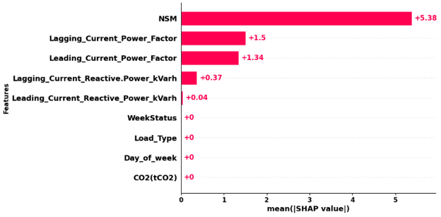
Figure 5. SHapley Additive exPlanation (SHAP) feature importance analysis
To analyze the important features of the data, SHAP is employed to elucidate the characteristics of the clusters within the dataset [35]. Figure 5 plots a succinct and comprehensible explanation of these clusters by identifying which features exerted the most significant influence on the clustering outcome and detailing each feature's specific contribution to the predicted cluster for every training sample. The NSM feature stands out as the most significant, with a mean SHAP value of +5.38, indicating its strong positive contribution to the model's predictions.
Following this, Lagging_Current_Power_Factor and Leading_Current_Power_Factor features also show notable positive impacts with mean SHAP values of +1.5 and +1.34, respectively. Lagging_Current_Reactive_Power_kVarh and Leading_Current_Reactive_Power_kVarh features contribute less, with values of +0.37 and +0.04. Conversely, features such as WeekStatus, Load_Type, Day_of_week, and CO2(tCO2) features exhibit a mean SHAP value of +0, suggesting they have negligible or no average impact on the model's predictions within this context. Based on these results, two models will be used to develop the prediction model based on the DNN approach. The purpose of that is to explore the explainability and refinement of the data.
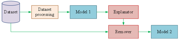
Figure 6 shows the idea of the two models. Model 1 utilized the completed dataset after processing, whereas Model 2 utilized the dataset after analyzing it by SHAP in the Explanator. The output of the Explanator, likely insights or identified features, goes into a remover to remove it from the dataset. Finally, the refined data from the remover is passed to Model 2, training a new model on the modified dataset, to improve performance and robustness based on the explainability insights. While the first and second models have the same architecture, the number of input features is different because the remover removes the less influential features.
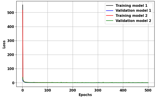
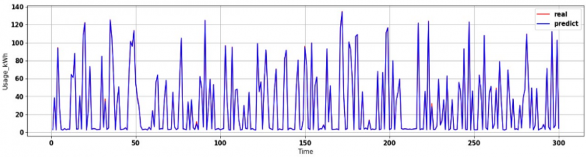
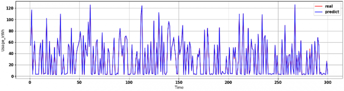
Figure 7 depicts the learning curve of the DNN algorithm for Model 1 and Model 2, where training and validation loss converge after 25 epochs. Figure 8 shows a comparison graph for 300 samples between the predicted energy generated by the proposed DNN of Model 1 and Model 2 in comparison with the real data for the testing set of data.
Figure 6. Structure of two deep neural network (DNN) models based on input dataset
Figure 7. Learning curve for Model 1 and Model 2
Figure 8 shows that the model yields an excellent fidelity in replicating true energy usage data for both models, which indicates its superior predictive performance. Moreover, based on Table 5, it becomes apparent that Model 2, based on the SHAP approach, achieves the same results as Model 1, where the value of the measured index, including RMSE, MAE, and CV, is the same for both training and testing. This means that SHAP is successfully able to identify the most important features, and the removed feature from the dataset does not affect the output result.
(a) The predicted energy consumption of Model 1 and the real data
(b) The predicted energy consumption of Model 2 and the real data
Figure 8. Comparison graph between the predicted energy consumption and the real data
Table 5. Performance evaluation between Model 1 and Model 2
|
Model |
Data |
|
Performance Index |
|
|
|
RMSE |
MAE |
Std |
CV |
||
|
Proposed DNN Model 1 |
Training |
0.32 |
0.21 |
0.4979 |
1.22 |
|
Testing |
0.31 |
0.21 |
0.5510 |
1.22 |
|
|
Proposed DNN Model 2 |
Training |
0.32 |
0.21 |
0.6300 |
1.22 |
|
Testing |
0.31 |
0.21 |
0.6134 |
1.22 |
|
Table 6. Performance evaluation of the prediction models and other models
|
Model |
Data |
Performance Index |
|
|
|
RMSE |
MAE |
CV |
||
|
SVM [11] |
Training |
1.89 |
1.51 |
6.92 |
|
Testing |
1.97 |
1.71 |
7.16 |
|
|
KNN [11] |
Training |
1.59 |
0.75 |
5.81 |
|
Testing |
2.99 |
1.75 |
10.90 |
|
|
RF [11] |
Training |
0.50 |
0.14 |
1.85 |
|
Testing |
1.12 |
0.36 |
4.09 |
|
|
Proposed DNN Model2 |
Training |
0.32 |
0.21 |
1.22 |
|
Testing |
0.33 |
0.21 |
1.22 |
|
In addition, a comparative study is conducted between the proposed DNN Model 2 and the results of the models that were obtained in the study [11] for predicting energy consumption. The evaluation criteria were the RMSE, the MAE, and CV. The evaluation results are listed in Table 6.
For example, in terms of training results, the results of the computer simulation reveal that the proposed DNN model reduced the value of the RMSE from 1.89 for SVM, 1.59 for KNN, and 0.5 for RF to 0.27 for the proposed DNN model. Besides, for the testing results, the proposed DNN model reduced the value of the RMSE from 1.97 for SVM, 2.99 for KNN, and 1.12 for RF to 0.31 for the proposed DNN model. These outcomes reveal that the proposed DNN model outperformed SVM, KNN, and RF in terms of prediction accuracy.
Efficient utilization of resources is important at every production stage. Estimation of the energy consumption is vital for sustainable resource allocation. AI has been extensively applied to enhance a wide range of issues in areas of industrial production. Among these issues, the analysis of the energy consumption profiles in industrial manufacturing is beneficial to enhance energy consumption. Integrating AI into prediction frameworks offers a substantial advancement in refining the precision and operational effectiveness of energy forecasting models. This work presents an implementation of a novel DNN prediction model for predicting energy consumption in the steel industry.
The proposed DNN model consisted of five layers arranged as stacked layers sequentially. Four activation functions (SiLU, ReLU, and linear activation function) were used sigmoid, to enhance the performance of the DNN prediction model. In terms of the data, two models were proposed. In the first model, the complete process data was used to train the model, whereas in the other model, the SHAP method was adopted to remove the unnecessary features from the dataset. By comparing the results of the two models, the SHAP method was useful for extracting important features from the data.
To evaluate the proposed DNN prediction model, a comparative study based on computer simulation shows that the proposed DNN approach has higher accuracy and better generalizability in the prediction of energy consumption compared with SVM, KNN, and RF methods.
The findings of this research help industrial manufacturing managers in making righteous decisions of selecting efficient energy management systems. Besides, adopting the SHAP method is useful for describing underlying relationships between features and outcome. However, a limitation of this study is that the dataset was collected from a single steel manufacturing plant, which may restrict the generalizability of the proposed model to other operational conditions and industrial environments. Future work will focus on validating the model using data from multiple plants and diverse operating scenarios to further assess and enhance its robustness and generalization capability.
[1] Qian, S., Li, L. (2023). A comparison of well-to-wheels energy use and emissions of hydrogen fuel cell, electric, LNG, and diesel-powered logistics vehicles in China. Energies, 16(13): 5101. https://doi.org/10.3390/en16135101
[2] Shalaeva, D.S., Kukartseva, O.I., Tynchenko, V.S., Kukartsev, V.V., Aponasenko, S.V., Stepanova, E.V. (2020). Analysis of the development of global energy production and consumption by fuel type in various regions of the world. IOP Conference Series Materials Science and Engineering, 952(1): 012025. https://doi.org/10.1088/1757-899x/952/1/012025
[3] Kapp, S., Choi, J., Hong, T. (2022). Predicting industrial building energy consumption with statistical and machine-learning models informed by physical system parameters. Renewable and Sustainable Energy Reviews, 172: 113045. https://doi.org/10.1016/j.rser.2022.113045
[4] Walther, J., Weigold, M. (2021). A systematic review on predicting and forecasting the electrical energy consumption in the manufacturing industry. Energies, 14(4): 968. https://doi.org/10.3390/en14040968
[5] Hao, X., Wang, Z., Shan, Z., Zhao, Y. (2018). Prediction of electricity consumption in cement production: A time-varying delay deep belief network prediction method. Neural Computing and Applications, 31(11): 7165-7179. https://doi.org/10.1007/s00521-018-3540-z
[6] Hasan, A., Nasser, A., Al-Araji, A., Shafiq, D., Al-Obaidi, A., Al-Khazraji, H., Humaidi, A. (2025). Enhanced product defect detection in smart manufacturing using ConvNeXt-stacked autoencoder architecture. Indonesian Journal of Science and Technology, 10(2): 297-316. https://doi.org/10.17509/ijost.v10i2.82229
[7] Abood, A.M., Nasser, A.R., Al-Khazraji, H. (2023). Predictive maintenance of electromechanical systems based on enhanced generative adversarial neural network with convolutional neural network. IAES International Journal of Artificial Intelligence, 12(4): 1704. https://doi.org/10.11591/ijai.v12.i4.pp1704-1712
[8] Nasser, A., Al-Khazraji, H. (2021). A hybrid of convolutional neural network and long short-term memory network approach to predictive maintenance. International Journal of Electrical and Computer Engineering, 12(1): 721. https://doi.org/10.11591/ijece.v12i1.pp721-730
[9] Mohd Kamal, M.H., Emar Azami, K.A. (2024). Image recognition for bearing fault detection based on convolutional neural network. Jurnal Mekanikal, 47(2): 101-108. https://doi.org/10.11113/jm.v47.476
[10] Al-Khazraji, H., Nasser, A., Khlil, S. (2022). An intelligent demand forecasting model using a hybrid of metaheuristic optimization and deep learning algorithm for predicting concrete block production. IAES International Journal of Artificial Intelligence, 11(2): 649. https://doi.org/10.11591/ijai.v11.i2.pp649-657
[11] Sathishkumar, V.E., Lim, J., Lee, M., Cho, K., Park, J., Shin, C., Cho, Y. (2020). Industry energy consumption prediction using data mining techniques. International Journal of Energy, Information and Communications, 11(1): 7-14. https://doi.org/10.21742/ijeic.2020.11.1.02
[12] Afzal, S., Ziapour, B.M., Shokri, A., Shakibi, H., Sobhani, B. (2023). Building energy consumption prediction using multilayer perceptron neural network-assisted models; comparison of different optimization algorithms. Energy, 282: 128446. https://doi.org/10.1016/j.energy.2023.128446
[13] Mahjoub, S., Chrifi-Alaoui, L., Marhic, B., Delahoche, L. (2022). Predicting energy consumption using LSTM, Multi-Layer GRU and Drop-GRU neural networks. Sensors, 22(11): 4062. https://doi.org/10.3390/s22114062
[14] Dinmohammadi, F., Han, Y., Shafiee, M. (2023). Predicting energy consumption in residential buildings using advanced machine learning algorithms. Energies, 16(9): 3748. https://doi.org/10.3390/en16093748
[15] Pham, A., Ngo, N., Truong, T.T.H., Huynh, N., Truong, N. (2020). Predicting energy consumption in multiple buildings using machine learning for improving energy efficiency and sustainability. Journal of Cleaner Production, 260: 121082. https://doi.org/10.1016/j.jclepro.2020.121082
[16] Hosseini, E., Saeedpour, B., Banaei, M., Ebrahimy, R. (2025). Optimized deep neural network architectures for energy consumption and PV production forecasting. Energy Strategy Reviews, 59: 101704. https://doi.org/10.1016/j.esr.2025.101704
[17] Agritania, M.M., Isnaini, M.M. (2025). Development of an engineering drawing detection and extraction algorithm for quality inspection using deep neural networks. Procedia CIRP, 132: 135-140. https://doi.org/10.1016/j.procir.2025.01.023
[18] Nele, L., Mattera, G., Vozza, M. (2022). Deep neural networks for defects detection in gas metal arc welding. Applied Sciences, 12(7): 3615. https://doi.org/10.3390/app12073615
[19] Yi-Fan, C., Yi-Kuei, L., Cheng-Fu, H. (2021). Using deep neural networks to evaluate the system reliability of manufacturing networks. International Journal of Performability Engineering, 17(7): 600. https://doi.org/10.23940/ijpe.21.07.p4.600608
[20] Albini, E., Long, J., Dervovic, D., Magazzeni, D. (2022). Counterfactual shapley additive explanations. In FAccT'22: Proceedings of the 2022 ACM Conference on Fairness, Accountability, and Transparency, Seoul, Republic of Korea pp. 1054-1070. https://doi.org/10.1145/3531146.3533168
[21] Lundberg, S., Lee, S.I. (2017). A unified approach to interpreting model predictions. arXiv preprint arXiv:1705.07874. https://doi.org/10.48550/arXiv.1705.07874
[22] Al-Badri, K., Dulaimi, H., Al-Khazraji, H., Humaidi, A.J. (2025). Adaptive neural network control for load-varying two-link robots using honey badger optimization. Journal of Robotics and Control, 6(2): 1061-1068. https://doi.org/10.18196/jrc.v6i2.26370
[23] April, A.A., Basu, J.K., Bhattacharyya, D., Kim, T. (2010). Use of artificial neural network in pattern recognition. International Journal of Software Engineering and Its Applications, 4(2): 23-34. https://doi.org/10.3390/polym14224876
[24] Abiodun, O.I., Jantan, A., Omolara, A.E., Dada, K.V., Mohamed, N.A., Arshad, H. (2018). State-of-the-art in artificial neural network applications: A survey. Heliyon, 4(11): e00938. https://doi.org/10.1016/j.heliyon.2018.e00938
[25] Albeiruti, H.A. (2025). Artificial intelligence for EEG analysis: A comprehensive review of deep learning techniques. Iraqi Journal of Computers, Communications, Control and Systems Engineering, 25(2): 9. https://doi.org/10.33103/uot.ijccce.25.2.9
[26] Mishra, C., Gupta, D.L. (2017). Deep machine learning and neural networks: An overview. IAES International Journal of Artificial Intelligence, 6(2): 66. https://doi.org/10.11591/ijai.v6.i2.pp66-73
[27] Lv, Q., Zhang, S., Wang, Y. (2022). Deep learning model of image classification using machine learning. Advances in Multimedia, 2022(1): 3351256. https://doi.org/10.1155/2022/3351256
[28] Talib, M.M., Sadik, M. (2025). Intelligent power management model for buildings using deep neural networks. Iraqi Journal of Computers, Communications, Control and Systems Engineering, 25(1): 2. https://doi.org/10.33103/uot.ijccce.25.1.2
[29] Salim, S.K., Msallam, M.M., Olewi, H.I. (2024). Design novel CNN architecture to protect personal devices from unauthorized access using face recognition. Nanotechnology Perceptions, 3(3): 82-93. http://doi.org/10.62441/nano-ntp.v20i3.7
[30] Elfwing, S., Uchibe, E., Doya, K. (2018). Sigmoid-weighted linear units for neural network function approximation in reinforcement learning. Neural Networks, 107: 3-11. https://doi.org/10.1016/j.neunet.2017.12.012
[31] Canchola, J.A., Tang, S., Hemyari, P., Paxinos, E., Marins, E. (2017). Correct use of percent coefficient of variation (% CV) formula for log-transformed data. MOJ Proteomics & Bioinformatics, 6(4): 316-317. https://doi.org/10.15406/mojpb.2017.06.00200
[32] Msallam, M.M., Alawad, N., Al Mhdawi, A.K., Al-Khazraji, A., Husain, S.S., Huamidi, A.J. (2024). ANN-based ship maneuvering motion control. In 8th IET Smart Cities Symposium (SCS 2024), Hybrid Conference, Bahrain, pp. 650-655. https://doi.org/10.1049/icp.2025.0866
[33] Öter, A., Ersöz, B. (2025). Artificial intelligence assisted solar energy forecasting by explainability approaches with LIME and SHAP. El-Cezeri, 12(2): 205-212. https://doi.org/10.31202/ecjse.1591721
[34] AL-Ali, M.A., Lutfy, O.F., Al-Khazraj, H. (2024). Comparative study of various controllers improved by swarm optimization for nonlinear active suspension systems with actuator saturation. International Journal of Intelligent Engineering & Systems, 17(4): 870-881. https://doi.org/10.22266/ijies2024.0831.66
[35] Nohara, Y., Matsumoto, K., Soejima, H., Nakashima, N. (2022). Explanation of machine learning models using shapley additive explanation and application for real data in hospital. Computer Methods and Programs in Biomedicine, 214: 106584. https://doi.org/10.1016/j.cmpb.2021.106584