Sayadi Ahmed | Djekidel Rabah* | Bessidik Sid Ahmed | Hamed D. Al-Sharari | Khalil Algarny | Sherif S. M. Ghoneim
© 2026 The authors. This article is published by IIETA and is licensed under the CC BY 4.0 license (http://creativecommons.org/licenses/by/4.0/).
OPEN ACCESS
The objective of this research is the analysis and mitigation of the electromagnetic fields emanating from the ultra-high-voltage (UHV) transmission line installed in a delicate location. The approach involves employing a hybrid technique that integrates the current simulation technique (CST) with the equilibrium optimizer (EO) algorithm in determining the optimal design of compensating devices. This includes the optimal number of filamentary currents, passive loop dimensions, and the necessary capacitor sizes. The results show that the magnetic induction follows a Gaussian distribution centered on the power line axis and decreases with lateral distance. The optimized passive compensation loops significantly reduce the magnetic field along the corridor. A single passive loop achieves a maximum reduction of 40.64%, while a double passive loop provides a higher attenuation of up to 60.34%. In conclusion, the double passive loop configuration offers the most effective solution for magnetic field mitigation. Furthermore, the comparison between CST-based simulations and transmission line analytical results demonstrates excellent agreement, confirming the validity of the proposed approach.
modelling, optimization, equilibrium optimizer algorithm, ultra-high-voltage overhead transmission line, magnetic induction, mitigation loop
Electricity plays a fundamental role in modern society by improving living conditions, meeting basic needs, and supporting sustainable development. It is also a key driver of economic and social progress, and per capita energy consumption is commonly used as an indicator of a country's level of development [1, 2]. Global electricity demand continues to increase due to rapid economic growth, industrial expansion, population growth, and urbanization. To meet these growing needs, power systems must be expanded and upgraded with more efficient extra-high and ultra-high voltage transmission infrastructures. Electrical energy generated in power plants is delivered to consumers through interconnected grids composed of transmission lines, substations, and distribution systems [3, 4].
Over the past four decades, increasing attention has been given to the potential impacts of electric and magnetic fields (EMFs) emitted by high-voltage power transmission lines on human health and the environment. Studies conducted by international organizations, including the World Health Organization (WHO), indicate that exposure to EMFs can induce electric currents in the human body, potentially leading to biological effects such as tissue heating, stimulation of the nervous system, and visual disturbances [5-8].
Some epidemiological studies suggest a possible association between long-term exposure to power-frequency magnetic fields and childhood leukemia, although evidence for adults remains inconclusive [9-11]. In addition to human health concerns, EMFs may also affect wildlife, particularly avian species, influencing their reproductive biology and behavior [12, 13]. Despite extensive theoretical and experimental investigations, significant scientific uncertainties remain regarding the long-term effects of EMF exposure [14-16].
From a public health perspective, these uncertainties have led many countries to adopt precautionary approaches aimed at minimizing exposure levels, especially in residential and sensitive areas [17-20].
In order to mitigate risks, there are international guidelines that restrict human exposure to EMFs. ICNIRP, an organization recognized by the WHO, suggests that maximum exposure to electric fields should not exceed 5 kV/m and to magnetic fields should not be more than 200 µT for the general population, while for occupational exposure, maximum limits are 10 kV/m and 1 mT [21-23].
These guidelines have been adopted by many countries as national standards. However, some countries enforce stricter limits, particularly in densely populated areas, near schools, and around hospitals, to ensure higher levels of protection [24-26]. The variation in international policies reflects the ongoing debate regarding the biological effects of low-frequency electromagnetic fields and the need for precautionary measures.
Considering the problems associated with the EMF effects, it becomes necessary to analyze and model the magnetic fields produced by the high-voltage transmission lines accurately. There are different mathematical models developed for determining the magnetic field distribution along overhead lines. These include the Biot-Savart law approach, current simulation methods, and finite element methods [27-33].
To reduce EMF exposure, various mitigation techniques have been proposed. These include both passive shielding methods, such as passive loop conductors and optimized conductor arrangements, and active shielding techniques, which use controlled currents to counteract magnetic fields [30-33]. Due to their low cost and ease of deployment, passive loop systems remain the most widely studied configurations in this category.
Numerous studies have investigated the effectiveness of passive shielding configurations for magnetic field reduction [34-42]. However, most existing works primarily focus on single-loop compensation strategies, with limited comparative analysis of double-loop configurations and their performance under different operating conditions.
The design of effective shielding systems requires solving complex optimization problems involving multiple parameters such as loop position, geometry, and current. Traditional optimization methods have been widely applied, including genetic algorithms, simulated annealing, and particle swarm optimization [36-40].
More recently, metaheuristic optimization techniques have significantly improved the performance and robustness of magnetic shielding designs. A variety of algorithms have been developed for addressing such challenges, among which the equilibrium optimizer (EO) algorithm is considered a very promising approach. The EO algorithm was put forward by Faramarzi et al. [43] in 2020 and is based on the behavior of particles that tend to achieve equilibrium in a chemical system. This algorithm has proved to be highly useful in addressing various types of optimization problems encountered in engineering contexts.
The objective of this paper is to construct an appropriate model for calculating the magnetic field produced by single and double-circuit overhead ultra-high voltage transmission lines, along with devising an appropriate strategy for mitigating these magnetic fields. Numerical simulations are carried out using a hybrid approach that combines the current simulation technique (CST), well-suited for modeling bundled conductors used in ultra-high-voltage (UHV) transmission systems, with a metaheuristic optimization algorithm [44]. The surface current distribution within each of the sub-conductors of the bundle conductor is modeled as a finite number of filamentary current distributions over an imaginary internal surface. The location and number of such filaments are optimized in order to satisfy certain boundary conditions via the EO algorithm [45, 46].
To mitigate magnetic fields near transmission lines, passive shielding loops made of conductive or magnetic materials can be installed beneath the phase conductors. Through electromagnetic induction, currents induced in these closed loops generate secondary magnetic fields that partially oppose the original field [47, 48]. The geometric and electrical parameters of these compensation loops are optimized using EO to enhance shielding performance. Finally, the results are validated by comparison with the multi-conductor transmission line method.
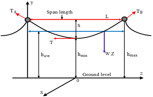
In the field of rational mechanics, a flexible overhead conductor suspended between two supports of equal elevation and subjected to its own uniformly distributed weight assumes the geometric profile of a catenary (see Figure 1). The sag (S) is the vertical distance between the conductor’s lowest point and the midpoint of the span, while L denotes the span length between suspension points. For mathematical modeling, the catenary is commonly approximated by a parabolic curve [49, 50]. The mathematical equation that represents the parabola is given by the following form [51-53]:
$y(z)=h_{\min}+\left(\frac{2 Z}{L}\right)^2 \times S$ (1)
where, $h_{\min}$ is the lowest ground clearance in the middle of the span, S is the highest sag of the conductor, L is the length of the conductor, and z is the point along the span length where the conductor is longest.
Figure 1. Simplification of longitudinal geometry of conductor power line
In practice, the conductor height above ground varies along the span and depends on weather conditions. To simplify overhead line geometry, an average height is defined, assuming the conductor is horizontal and parallel to flat ground. This approximation facilitates field calculations and is determined using the following equation [53, 54]:
$h_{\text {ave}}=h_{\max}-\frac{2}{3} \times S$ (2)
In this context, $h_{\max}$ represents the peak elevation of the conductor above the ground surface.
The maximum sag of the parabola can be calculated using the following formula [51-53]:
$S=\frac{W L^2}{8 T}$ (3)
where, $W$ is the weight per unit length of the conductor; $T$ is the tension in the conductor; $L$ is the horizontal distance between the two towers.
The ground plays a crucial role in studying overhead power transmission lines, acting as a return path for current and influencing the distribution of electromagnetic fields, as it constitutes a boundary interface between two different media. Modeling ground effects generally relies on two main assumptions. In the case of perfectly conductive soil, electromagnetic fields are completely reflected without penetrating the ground. This assumption allows the use of image theory, which considerably simplifies calculations by replacing the ground effect with frequency-independent equivalent sources. Conversely, for real soil with finite conductivity, electromagnetic fields partially penetrate the ground to a certain depth that depends primarily on the source frequency, where the fields are subject to attenuation and phase shift [55-57].
In magneto-statics, the magnetic field calculation is generally based on Beau-Savart's law. This physical law explains how an electric current (Ic) flowing in a straight wire generates a magnetic field at a precise point in space located at a distance (d) from the current source; this field is calculated as follows [58, 59]:
$B_T=\frac{\mu_0}{2 \pi} \frac{I_c}{d}$ (4)
The current flowing through the wire is $I_c$, the distance between the conductor and the point where the magnetic field is calculated is d, and the magnetic permeability of free space is $\mu_0$.
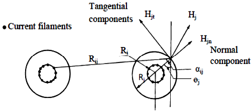
Figure 2. The normal and tangential components of the field at a point on the surface of the sub-conductor
For very high-voltage three-phase overhead transmission lines, conductor bundles are widely used to improve energy efficiency. These bundles consist of several symmetrically arranged sub-conductors per phase, electrically connected so that the current is evenly distributed among them. As a result, the current in each sub-conductor remains constant and proportional to the total phase current [49]. In this context, the CST, derived from the Biot-Savart law, is an efficient method for calculating magnetic induction. It offers the advantage of solving a reduced number of linear equations. In this method, the actual surface current of each sub-conductor is represented by discrete filamentary currents distributed over a fictitious cylindrical surface within the conductor (see Figure 2) [60-64]. The number and placement of filament currents in the simulation are not random but depend on the number and spatial configuration of the conductors and must meet the following requirements:
1. The normal component of the magnetic field at the surface of the conductor is zero.
2. The sum of the filament current simulation of the conductor should be equivalent to the current intensity of the conductor itself.
In considering the earth as a perfect conductor, the influence of the earth can be simulated by introducing image currents of the ground plane at a complex penetration depth in the opposite direction of the source currents [45-48].
In order to determine the current densities in the filaments, a system of equations is set up for as many contour points on the surface of the conductors as there are unknown current densities to meet the boundary conditions below [60-64].
$\begin{aligned} \sum_{i=1}^{N_C \times n_f \times m_s} k_{I J} I_i & =0, j \quad=1,2, \ldots \ldots,\left(N_C \times m_s\right) \times\left(n_f\right.-1) \\ \sum_{i=(q-1) n_f+1}^{n_f \times q} I_i & =I_{c q}, q=1,2, \ldots \ldots,\left(N_C \times m_s\right)\end{aligned}$ (5)
where, $n_f$ denotes the number of filamentary line currents, $N_C$ represents the number of power line conductors; $m_s$ is the number of sub-conductors per phase. $K_{i j}$ the coefficient of normal magnetic field depends on the coordinates of the contour point $i^{\text {th }}$ and the filamentary current point $j^{\text {th }}$ it is expressed by [60-64]:
$k_{I J}=\frac{\mu_0}{2 \pi} \ln \frac{R_j}{R_{i j}}$ (6)
$R_{i j}$ is the distance between the simulation current point (i) and the contour point (j) at the surface of the sub-conductor. $R_j$ is the imaginary radius of the filamentary current point.
After determining the equivalent currents representing the currents flowing through the transmission line conductors by solving the aforementioned system of linear equations, the corresponding magnetic potential can be estimated according to the following equation [60-64]:
$\begin{aligned} A_{I J}=\frac{\mu_0}{2 \pi} \sum_{i=(q-1) n_f+1}^{n_f \times q} & I_i k_{I J}, q\quad=1,2, \ldots \ldots,\left(N_C \times m_s\right)\end{aligned}$ (7)
To ensure accurate results, the calculated filament currents must be validated. First, several verification points are selected on the conductor surface, and the magnetic potential is recalculated. The relative error between the computed magnetic potential and the actual potential applied to the energized conductor is subsequently evaluated to assess the accuracy of the simulation.
Using the superposition principle in Cartesian coordinates, the horizontal and vertical components of the magnetic induction generated by the line currents at a given point can be determined using the following equations [65-67].
$\begin{gathered}B_x=-\frac{\mu_0}{2 \pi} \sum_{\substack{i=1}}^{N_C \times n_f \times m_s} I_i\left[\frac{y_i-y_j}{r_{i j}{ }^2}-\frac{y_i+y_j+D_e}{r_{i j}{ }^{\prime 2}}\right] \\ B_x=\frac{\mu_0}{2 \pi} \sum_{i=1}^{N_C \times n_f \times m_s} I_i\left[\frac{x_i-x_j}{r_{i j}{ }^2}-\frac{x_i-x_j}{r_{i j}{ }^{\prime 2}}\right]\end{gathered}$ (8)
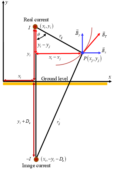
In this context, $I_i$ represents the current flowing through the conductors of the power line; $r_{i j}$ is the distance between each conductor and the desired point $(\mathrm{P})$; $r_{i j}^{\prime}$ is the distance between each image conductor and the desired point $(\mathrm{P})$; $D_e$ is the complex penetration depth as illustrated by Figure 3, and is given by the following expression [67]:
$D_e=\sqrt{2} \delta e^{-j \frac{\pi}{4}}, \delta=\sqrt{\frac{\rho_s}{\pi f \mu_0}}$ (9)
where, $\rho_s$ denotes the soil resistivity, $f$ is the frequency of the current source, and $\delta$ represents the earth skin depth of the ground.
When calculating the magnetic field above perfectly conductive soil, the return current induced in the ground must be considered. This is modeled as an image current located below the surface at a depth equal to the conductor height plus the penetration depth, which depends on soil resistivity and frequency. Total magnetic induction is obtained by summing the components, as described in this equation [65-68].
$B_t=\sqrt{\left(B_x\right)^2+\left(B_y\right)^2}$ (10)
Figure 3. The magnetic field generated around a current traversing a conductor
It should also be noted that in this magnetic field assessment, the induced current in the earth wire resulting from the current effect that passing in the overhead conductor can be taken into consideration. It can be calculated using the equation below [53, 54]:
$\left[I_g\right]=\left[Z_{g g}\right]^{-1}\left[Z_{g p}\right]\left[I_p\right]$ (11)
where, $I_g$ represents the vector of earth wires induced currents; $I_p$ represents the vector of currents in the phase conductors; $Z_{g g}$ is the matrix of self-impedance of the earth wires; $Z_{g p}$ is the matrix of mutual impedances between earth wire and each phase conductor.
The self and mutual impedances per unit length can be obtained using Carson’s equations with ground return concept, as indicated below [69, 70]:
$Z_{g g}=R_{g g}+j \omega \frac{\mu_0}{2 \pi} \ln \left(\frac{D_e}{r_{g g}}\right)$ (12)
where, $R_g$ is the resistance per unit length of earth wire; $d_{g p}$ is the mutual distance between phase conductor and earth wire; $r_{g g}$ is the geometrical mean radius of earth wire.
Mitigation strategies aimed at reducing magnetic induction fall into two distinct approaches. Passive compensation relies on generating an induced current in a conductive loop under the influence of the power line. Active compensation, on the other hand, involves injecting a current, using an externally powered coil, with its amplitude and phase appropriately adjusted [71-74].
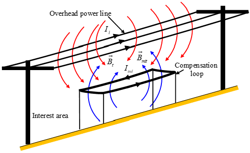
Figure 4. Arrangement of three-phase overhead power line conductors and a passive compensation loop
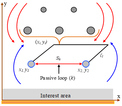
Passive magnetic compensation involves installing one or more short-circuited conductive loops beneath overhead power conductors (see Figure 4). Electromagnetic induction from the line currents generates induced currents in these loops, producing a secondary magnetic field that opposes the main field and reduces its intensity in the protected area [34-42]. According to Faraday’s law, time-varying currents in the overhead conductors create a changing magnetic flux through the loop, inducing an electromotive force (EMF). In practice, this induced EMF is treated as an induced voltage, described by the following mathematical expression [36-42, 72-79].
$V_{i n d}=-\frac{d_{\emptyset l}}{d t}=j \omega \emptyset_l$ (13)
In this expression, $V_{\text {ind}}$ represents the induced EMF within the closed loop, while $d_{\varnothing l}$ denotes the variation in magnetic flux penetrating the circuit over time, and ω is the angular frequency. The negative sign indicates the application of Lenz’s law to mathematics, as it shows the direction in which the polarity of the generated voltage should oppose the change in the magnetic flux that caused it.
The magnetic flux created by the sinusoidal change in the currents flowing in the conductor wires of the overhead power lines across the surface of the closed path can be obtained using the following equation [36-42, 72-79]:
$\emptyset_l=\iint \vec{B}_t d \vec{s}$ (14)
where, $\vec{B}_t$ is the magnetic induction vector at the given point; $d \vec{s}$ is an elemental area vector on the given surface.
It should be noted, as shown in Figure 4, that the magnetic compensation loop plane is placed parallel to the phase conductors of the power line; therefore, only the vertical component of the magnetic field crosses the surface of the loop and contributes to the magnetic flux calculation. Consequently, the previous equation of magnetic flux can be simplified as follows [36-42, 72-79]:
$\emptyset_l=l_l \int_{x_1}^{x_2} \vec{B}_y d \vec{x}$ (15)
where, $l_l$ is the compensation passive loop length.
The two conductors of the passive compensation loop are positioned at (x₁, y₁) and (x₂, y₂) beneath the overhead phase conductors. Considering the effect of ground-induced currents on the power line’s magnetic field, the resulting magnetic flux leakage is expressed as follows [72-79]:
$\begin{aligned} \emptyset_l=-\frac{\mu_0 l_1}{4 \pi} \sum_{i=1}^n I_i & \ln \frac{\left[\left(x_2-x_i\right)^2+\left(y_i-y_2\right)^2\right]}{\left[\left(x_1-x_i\right)^2+\left(y_i-y_1\right)^2\right]}\times \frac{\left[\left(x_1-x_i\right)^2+\left(y_i+y_1+D_e\right)^2\right]}{\left[\left(x_2-x_i\right)^2+\left(y_i+y_2+D_e\right)^2\right]}\end{aligned}$ (16)
The per-unit-length self-impedance $Z_{\text {loop }}$ of a magnetic compensation loop is represented as the series combination of its resistance $R_l$, self-inductance $L_l$, and distributed capacitance $C_l$. It is generally calculated using the following formula [41, 42]:
$Z_{\text {loop }}=R_l+j\left(\omega L_1-\frac{1}{\omega C_1}\right)$ (17)
The self-inductance of a closed compensation loop depends on its geometry, with two conductors separated by a distance $S_k$ and each having a radius $r_l$. The inductance is calculated using the following expression [36-42, 72-79].
$L_l=\frac{\mu_0}{\pi} \ln \frac{S_k}{r_l}$ (18)
where, $r_l$ is the radius of the loop's conductor; $S_k$ is the horizontal distance separating the passive loop conductors (see Figure 5).
The compensating magnetic field is proportional to the induced current in the loop, which is limited by the loop’s impedance. To increase this current, a series compensating capacitor is added to reduce the inductive reactance, with its capacitance carefully selected. The induced loop current is determined from the following relationship [36-42, 72-79]:
$I_{\text {ind}}=\frac{V_{\text {ind}}}{Z_{\text {loop}}}$ (19)
Figure 5. Mitigation of magnetic induction by a passive compensating loop
The induced current generates a magnetic field that counteracts the magnetic field produced by the source current.
For a geometric closed loop with the coordinates of the conductors $\left(x_k, y_k\right)$ and the observation point $\left(x_j, y_j\right)$, the amplitude of the compensation magnetic field can be written in the analytical form as follows [79-81]:
$B_{m i t}=\frac{\mu_0}{2 \pi} \sum_{k=1}^n I_{i n d}\left[\frac{\left(x_j-x_k\right) i+\left(y_j-y_k\right) j}{\left(x_j-x_k\right)^2+\left(y_j-y_k\right)^2}\right]$ (20)
The resultant magnetic field is obtained as the vector sum of the primary field and the field generated by the closed loop, and can be expressed as follows [69-72]:
$\vec{B}_{r e s}=\vec{B}_t+\vec{B}_{m i t}$ (21)
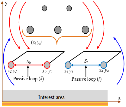
For two adjacent closed compensation loops of the same conductor type (Figure 6), electromagnetic induction causes each time-varying induced current to generate a magnetic flux in the other loop, producing an EMF. This mutual induction depends on the distance between the loop conductors, the geometry of each loop, and the conductor material [37-40, 72-82].
Figure 6. Mitigation of magnetic induction by two passive compensating loops
The values of the self and mutual coupling impedances of the compensation loops are calculated from the equations given below [37-40, 72-82]:
$\left.\begin{array}{l}Z_{k k}=R_l+j\left(\omega \frac{\mu_0}{\pi} \ln \frac{S_k}{r_l}-\frac{1}{\omega C_k}\right) \\ Z_{k l}=j \omega \frac{\mu_0}{\pi} \ln \left(\frac{d(k 1, l 2) \cdot d(k 2, l 1)}{d(k 1, l 1) \cdot d(k 2, l 2)}\right) \\ Z_{l k}=j \omega \frac{\mu_0}{\pi} \ln \left(\frac{d(k 2, l 1) \cdot d(k 1, l 2)}{d(k 1, l 1) \cdot d(k 2, l 2)}\right) \\ Z_{l l}=R_l+j\left(\omega \frac{\mu_0}{\pi} \ln \frac{S_l}{r_l}-\frac{1}{\omega C_l}\right)\end{array}\right\}$ (22)
At power frequency, mutual induction governs the behavior of compensation loops, as induced currents are significant and the effect of mutual capacitance on mutual impedance can be neglected. After computing self and mutual impedances, the induced currents and compensating magnetic field are determined as previously described. The effectiveness of the magnetic compensation is quantified by the shielding or reduction coefficient, defined as the ratio of the principal magnetic field before and after compensation at the same point [37, 82, 83].
$S_c=\frac{B_t}{B_{\text {res}}}$ (23)
The EO is a metaheuristic algorithm inspired by dynamic equilibrium processes in physical systems, such as fluids. Proposed by Faramarzi et al. [43] in 2020, it efficiently solves complex optimization problems using a controlled attraction toward the best solutions, balancing exploration of new regions and exploitation around promising areas. The algorithm begins by generating an initial population randomly within the search space, forming the basis for iterative optimization toward the global optimum [84-87].
$C_i^d=C_{\min }+\operatorname{rand}_i^d\left(C_{\max }+C_{\min }\right)~i=1,2, \ldots . . D$ (24)
The parameter D defines the number of dimensions, with $C_{\max}$ and $C_{\min}$ serving as the boundary limits for each dimension. The position of each individual particle (i) is represented by C, which is updated using a random vector rand generated within the range [0, 1].
Immediately afterward, the population will be estimated using the fitness function to assign the four best solutions obtained. The next step involves defining the equilibrium state of the algorithm, where five particles, the four best solutions, and their average are used to define the equilibrium pool according to the equation below [84-87]:
$\vec{C}_{e q, p o o l}=\left\{\vec{C}_{e q(1)}, \vec{C}_{e q(2)}, \vec{C}_{e q(3)}, \vec{C}_{e q(4)}, \vec{C}_{e q(a v e)}\right\}$ (25)
During the algorithm optimization process, an exponential term $F$ is constantly involved to maintain the balance between global and local search. It is defined as follows [84-87]:
$F=e^{-\lambda\left(t-t_0\right)}$ (26)
where, $\lambda$ is a random vector within the interval [0, 1]; $t$ denotes a non-linear function and is calculated by the following equation [84-87]:
$t=\left(1-\frac{\text { Iter}}{\text { MaxIter}}\right)^{\left(\alpha-\frac{\text { Iter}}{\text { MaxIter}}\right)}$ (27)
where, Iter is the current iteration; MaxIter is the maximum number of allowed iterations; $\alpha$ is a constant used to control the exploitation capacity; $t_0$ denotes a parameter used to improve exploration and exploitation capacities, it is defined by the equation given below [84-87]:
$t_0=\frac{1}{\lambda} \ln \left(-\beta \operatorname{sign}(r-0.5)\left[1-e^{-\lambda t}\right]\right)+t$ (28)
where, $r$ is a random vector in the interval [0, 1]; $\beta$ is a constant used to control the phase of the exploration capability. Often $\alpha$ and $\beta$ are taken to be equal to 1 and 2, respectively.
By replacing the parameter indicated in Eq. (28) into Eq. (26), the new exponential term becomes as follows [84-87]:
$F=\beta \operatorname{sign}(r-0.5)\left(e^{-\lambda t}-1\right)$ (29)
The generation rate $G$ is a key factor in the operation of the EO algorithm. It controls the search capacity, contributing to providing the best results through optimal performance of the exploitation phase, and is formulated by the following equation [84-87]:
$\vec{G}=\left\{\begin{array}{c}0.5 r_1(\vec{\lambda} \vec{C}) \vec{F}, r_2 \geq G P \\ 0 \quad, r_2<G P\end{array}\right\}$ (30)
where, $r_1$ and $r_2$ are random values between 0 and 1; $G P$ represents the generation rate and is set to 0.5. With this value, $G P$ creates the best balance between exploration and exploitation phases. The update rule of the EO algorithm is described as follows [77-80]:
$C=\vec{C}_{e q}+\left(\vec{C}-\vec{C}_{e q}\right) \vec{F}+\frac{\vec{G}}{\vec{\lambda} V}(1-\vec{F})$ (31)
The simplified basic pseudocode of the EO algorithm is described in Table 1 [88, 89].
Table 1. Pseudo-code of the basic equilibrium optimizer (EO) algorithm
|
Steps |
Pseudo-Code of Basic EO Algorithm |
|
1 |
Select initial parameters of algorithm, maximum number of iterations, parameters α, β, r, r1, r2, t, GP, number and limits of variables. |
|
2 |
Randomly initialize the number of populations (candidate solutions). |
|
3 |
Define and evaluate the objective function for all solutions. |
|
4 |
Select the four best solutions, calculate the average value and the equilibrium milieu using Eq. (25). |
|
5 |
For each solution, update according to the parameters of exponential term F and generation rate G mentioned in Eqs. (29) and (30), respectively. |
|
6 |
Update the solution (concentration) using Eq. (31) to generate a new solution. |
|
7 |
Evaluate the new solution and replace if improved. |
|
8 |
Update the Equilibrium Pool. Check if the stopping condition is satisfied; otherwise, the algorithm iterates from step (3). |
Under the CST, to determine the proper placement and number of line filamentary currents, the objective function employed in the optimization process could be formulated as the relative error of the magnetic vector potential as shown below [90]:
$O F=\frac{1}{n_f} \times \sum_{i=1}^{m \times n_f}\left|\frac{B_t\left(x_k, y_k\right)-B_{r e s}\left(x_k, y_k\right)}{B_t\left(x_k, y_k\right)}\right| \times 100$ (32)
where, $B_t$ is the magnetic induction produced by the power line at the given position (before compensation); $B_{\text {res}}$ is the resultant magnetic induction at the same position (after compensation).
The objective function employed to find the optimal coordinates of the closed loop conductors is given by [69]:
$O F=-\sqrt{B_t-B_{r e s}\left(x_K, y_k\right)^2}$ (33)
The negative sign shows the maximization of this objective function [53].
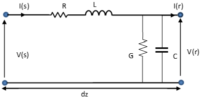
The transmission line approach allows us to study propagation phenomena along a conductor. It relies on solving two differential equations, known as the telegraph equations. An overhead power transmission line can be considered as a succession of circuits whose parameters are uniformly distributed along its entire length. These circuits consist of an infinite number of identical elements, such as linear resistances and inductances in the longitudinal direction and leakage conductance’s with linear capacitances in the transverse direction. As illustrated in Figure 7, the operation of the two-wire line per unit length is modeled by a line segment where the input voltage and current (source) are related to the output voltage and current (receiver) through the parameters of a two-port network A, B, C, and D, as shown below [91-94]:
$\begin{aligned} & V(s)=A V(r)+B I(r) \\ & I(s)=C V(r)+D I(r)\end{aligned}$ (34)
Figure 7. Simplified model of a medium-length electrical transmission line
The four parameters of the two-port network depend on the transmission line constants. A, B, C and D are characteristic parameters that depend on the transmission line constants R, L, C, and G. For a fully transposed three-phase system of average length, Z represents the series impedance of the system and Y its parallel admittance; they can be described by [91-94]:
$\begin{gathered}Z=R+j \omega L \\ Y=G+j \omega C\end{gathered}$ (35)
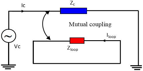
Placing a closed, two-conductor shielded loop beneath the transmission lines allows the induced current to be determined by the mutual coupling between the power line conductors and the loop, as illustrated in Figure 8.
Figure 8. Mutual coupling between a transmission conductor and a conductive loop
To analyze induced currents between parallel conductors, it is preferable to use admittances rather than impedances. For medium-length overhead lines, the parallel admittance mainly comprises a capacitive component, while the resistive (conductance) component is often negligible. The conductor’s admittance can be expressed as follows [95-97]:
$Y_c=\frac{R}{R^2+(\omega L)^2}-j\left(\frac{\omega L-\omega C\left(R^2+(\omega L)^2\right)}{R^2+(\omega L)^2}\right)$ (36)
The closed loop can be considered as a single equivalent conductor characterized by the total impedance mentioned in Eq. (18), and consequently, its admittance is expressed as follows [95-97]:
$Y_1=\frac{R_1}{\left(\omega L_1-\frac{1}{\omega C_1}\right)^2+R_1^2}-j \frac{\left(\omega L_1-\frac{1}{\omega C_1}\right)}{\left(\omega L_1-\frac{1}{\omega C_1}\right)^2+R_1^2}$ (37)
For a symmetrical three-phase system, a matrix of admittances can model the combined parameters of the overhead line and passive loop. In this approach, the passive loop is assumed de-energized. The resulting admittance matrix for the complete system, including line conductors and the passive loop, is expressed as follows [95-97]:
$\left[\begin{array}{c}I_c \\ I_e \\ I_{\text {loop }}\end{array}\right]=\left[\begin{array}{lll}Y_c & Y_{c e} & Y_{c l} \\ Y_{e c} & Y_{e e} & Y_{e l} \\ Y_{c l} & Y_{l e} & Y_{l l}\end{array}\right] \cdot\left[\begin{array}{c}V_c \\ V_e \\ V_{\text {loop }}\end{array}\right]$ (38)
In the first step, since the passive loop is not energized, the $V_{\text {loop}}$ voltage is equal to zero. Substituting this value into the admittance matrix, it can be deduced [95-97]:
$\left[V_e\right]=Y_{e e}^{-1}\left(I_e-Y_{e c} V_c\right)$ (39)
In the second step, it can be substituted the expression of the deduced voltage into the expression for the induced current in the loop, which gives the following [95-97]:
$I_{l o o p}=Y_{l c} V_c+Y_{l e}\left(Y_{e e}^{-1}\left(I_e-Y_{e c} V_c\right)\right)$ (40)
After rearranging the terms of this equation, it can be obtained [88-90]:
$I_{l o o p}=\left(Y_{l c}-Y_{l e} Y_{e c} / Y_{e e}\right) V_c+\left(Y_{l e} / Y_{e e}\right) I_e$ (41)
Figure 9. Configuration schematic of single circuit horizontal transmission power line
The magnetic field that is produced by the magnetic compensation coil can be determined after computing the induced current, as discussed previously from Eq. (21), along with the entire magnetic field of the whole electric system.
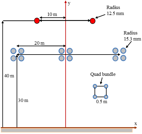
The analysis is done on a portion of a three-phase 1000 kV transmission line system that exhibits symmetry by having its phase conductors mounted horizontally with two ground wires (Figure 9). The phase voltage system is symmetrical and in positive sequence [98]. The line carries 5000 MW at a 0.9 power factor. The earth is assumed to be homogeneous with a resistivity of 100 Ω.m, and the system frequency is 50 Hz. DC resistance is 0.01 Ω/km for phase conductors and 0.063 Ω/km for earth wires. The mitigation loop conductors have a 1.25 cm radius, 0.225 Ω/km resistance. The length of the mitigation loop conductors and the transmission line segment is equal 1 Km.
In the first stage, calculate the induced current in the grounding cables using Eq. (11). As has been stated previously, this has to be done so that their impact can be considered in calculating the magnetic flux density.
$I_{g 1}=314.64 e^{j(142.18)^0}(A), I_{g 2}=309.1 e^{j(-6.41)^0}(A)$
Regarding the simulation approach employed in this numerical modeling, an appropriate selection of the number and spatial distribution of simulation current filaments is essential to meet the requirements of accuracy and computational efficiency. To counter this difficulty, an excellent performance optimization technique was chosen based on a fair comparison between several proposed algorithms, where the tests were repeated 10 times for each algorithm, with a maximum of 100 iterations. This simulation was programmed in the MATLAB (R2016b) environment on a Windows 11 operating system with an Intel (R) Core (TM) i5-1335U processor at 1.3 GHz and 16 GB of RAM. The parameter settings used for the competitive optimization algorithms are presented in Table 2.
Table 2. Parameter settings of the proposed algorithms
|
Methods |
Parameters Setting |
|
Equilibrium Optimizer (EO) Algorithm |
Npop = 20, α = 2; β = 1; GP = 0.5; r1, r2 [0, 1]. |
|
Firefly Algorithm (FA) |
Npop = 20; N = α = 0.4, β0 = 1, γ = 0.4 |
|
Grasshopper Optimization Algorithm (GOA) |
Npop = 20; F = 0.5; L = 1.5; Cmax = 1; Cmin = 0.00001. |
|
Grey Wolf Optimizer (GWO) |
Npop = 20, coef ϵ [0; 2], r1 and r2 ϵ [0; 1]. |
|
Particle Swarm Optimization (PSO) |
Npop = 20, c1 = 2, c2 = 2, w = 0.9. |
|
Genetic Algorithm (GA) |
Npop = 20, Pm = 0.2, Pc = 0.4. |
Figure 10. Variation of objective function with number of iterations for different proposed algorithms
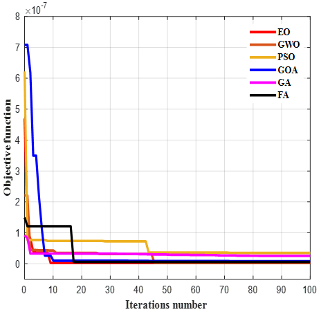
Figure 10 shows the convergence behavior of the objective function defined in Eq. (32). With respect to the number of iterations of the optimization algorithm. This process reflects the convergence of the optimization algorithms by minimizing the objective function, through a progressive decrease in the relative mean error, until the optimal solution is obtained in the considered search space. The best results obtained by these algorithms are listed in Table 3.
By comparing the performance of the different algorithms according to the criteria defined in Table 3, the following can be concluded: The EO algorithm achieved the best performance, with the lowest objective function value, the fastest convergence, and a relatively short execution time. The GWO algorithm offers similar accuracy but requires more iterations and a longer execution time. The PSO algorithm offers the fastest execution time, a slow convergence rate and lower resolution accuracy. The FA algorithm has demonstrated rapid convergence, but suffers from a high objective function value and a longer execution time. In contrast, the GOA and GA algorithms exhibited slower convergence and lower objective function values, making them less efficient and less effective. Indeed, the EO algorithm stands out as the most efficient and accurate, giving it a significant advantage for solving the problem under consideration.
Table 3. Comparison criteria between the adopted algorithms
|
Algorithms |
Objective Function Value |
Execution Time (s) |
Number of Convergence Iterations |
|
EO |
2.55e-09 |
422.275090 |
15 |
|
FA |
5.64e-09 |
1342.207265 |
25 |
|
GOA |
8.13e-08 |
2213.555260 |
78 |
|
GWO |
2.65e-09 |
556.817109 |
72 |
|
PSO |
3.47e-08 |
390.165797 |
72 |
|
GA |
2.52e-08 |
795.755906 |
75 |
Table 4 summarizes the best optimization results for the parameters that are incorporated into the simulation method and those obtained using the EO algorithm.
Table 4. Best values obtained by the equilibrium optimizer (EO) algorithm
|
|
Current Filaments Number |
Fictitious Conductor Radius (m) |
Objective Function Value |
|
Phase conductor |
37 |
0.1 |
4.1e-09 |
|
Ground wire |
38 |
0.008 |
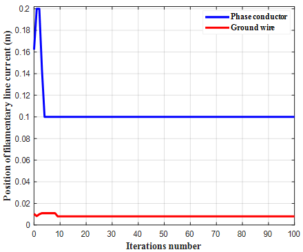
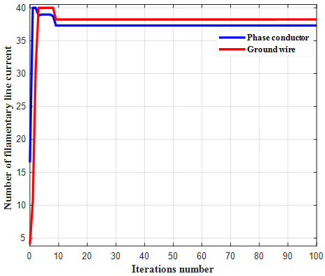
The optimum values of position and number of filaments of the simulation currents derived from the algorithm have been presented in Figures 11 and 12. This shows that the algorithm can find the optimum values very fast.
Figure 11. Convergence of currents filaments position towards the optimal values
Figure 12. Convergence of currents filaments number towards the optimal values
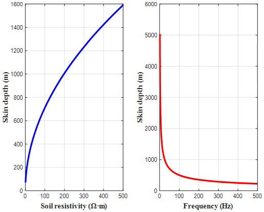
Figure 13. Penetration depth into the ground of magnetic field as a function of soil resistivity and current frequency
The variations in the depth of penetration of the magnetic field with respect to soil resistivity and frequency of the source current have been depicted in Figure 13, respectively. With the increase in soil resistivity, there is a gradual increase in the depth of penetration. On the other hand, an increase in resistivity causes a marked decrease in the depth of penetration.
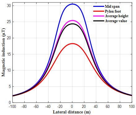
Figure 14 illustrates the lateral distribution of the magnetic field intensity at a height of 1 m above ground level. The field is strongest directly beneath the central phase conductor and drops off quickly as you move sideways across the right-of-way. Overall, the distribution forms a symmetric, bell-shaped, or Gaussian curve. This is explained by the fact that the conductors are horizontally aligned with regular spacing relative to the power line center, and that the contributions of each conductor are equal in magnitude and opposite in position.
Analysis of the simulated magnetic field reveals that the calculated magnetic field intensity for the power transmission line, taking into account its sag, is very high at the center and relatively low at its ends. This difference is due to the varying height of the conductors above the ground.
Figure 14. Distribution profile of magnetic induction at an elevation of 1 m above ground level
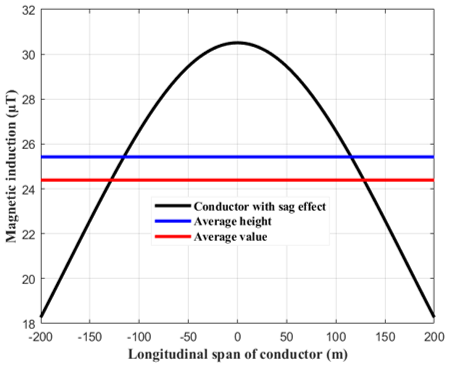
Without considering the sag, using the average conductor height, the calculated magnetic field strength falls between these two values and is approximately equal to the average value calculated by taking the sag into account, with a very small margin of error. The maximum values of magnetic field strength for the four states can be summarized in Table 5 below.
Table 5. Resulting maximum values for magnetic field strength at point (x = 0, y = 1 m)
|
|
Mid Span Length |
Pylon Foot |
Average Value |
Average Height |
|
Magnetic field strength (µT) |
30.51 |
18.27 |
24.39 |
25.42 |
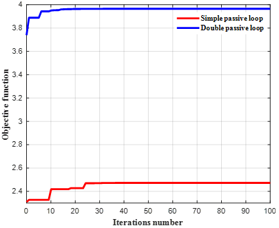
Figure 15 shows the longitudinal profile of the magnetic field distribution at a height of one meter from the ground level. Taking into consideration the conductor sag, the magnetic field intensity is highest at the center and then gradually decreases towards the edges, being lowest at the ends of the conductor. This demonstrates that the magnetic field distribution is not uniform throughout the power line. If the sag of the conductor is ignored, then the magnetic field intensity will be uniform across the entire length of the power line, and it will have a value equal to the average value if the conductor sag is considered. The magnetic field intensity is therefore dependent on the height of the conductor relative to the Earth's surface; that is, the higher the conductor height, the less the magnetic field intensity. The height of the conductor can be averaged out in order to simplify the calculation of the magnetic field of power transmission lines because its value will be roughly equal to that obtained when considering the conductor sag. To be able to have access to the optimal result of magnetic induction mitigation, it is first needed to optimize the coordinates of closed loops conductors and also compensation capacity value for the passive loop circuit with the help of a hybrid approach consisting of the suggested approach and EO. Figure 16 shows the optimization process of the objective function optimization, which is stated by Eq. (33), during a maximization process based on the number of iterations. It can be seen from this Figure that the values of the objective function increase with an increase in the number of iterations. This means that it gets closer to optimal values based on the size of the search space to keep magnetic induction in low levels. The optimization process takes place within a very small number of iterations in both cases of simple passive loop and double passive loop circuits.
Figure 15. Longitudinal magnetic induction profile at 1 m above ground level
Figure 16. Variation of the objective function as a function of the number of iterations
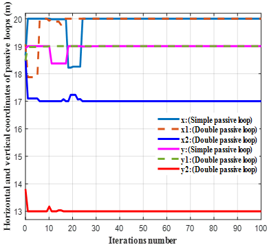
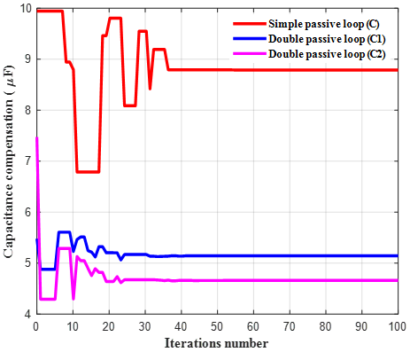
Figures 17 and 18 illustrate the results from the optimization technique (EO) for the optimum values of the parameters of the attenuation loop in relation to the coordinates of the conductors and combined capacitances; it can clearly be seen that the EO technique converges quickly towards the optimum values.
Figure 17. Variation of the coordinates values of the loops conductors with number of iterations
Figure 18. Optimal value of compensation series capacitance
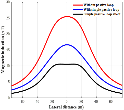
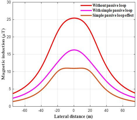
Figure 19 shows the lateral variation of the magnetic field at 1 meter above the ground level. By comparing the magnetic induction intensity before and after compensation using the simple passive loop, it is evident that there is a decrease in the magnetic field at each point along the overhead power line right-of-way. The decrease in the magnetic field was 34.66% for the midline right-of-way of the power line using the simple passive loop.
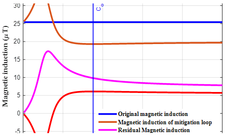
The parametric sweep of the magnetic induction variation at the point of symmetry (x = 0, y = 1 m) where the residual magnetic field is at its maximum as a function of the change in attenuation amplitude around its optimum value is depicted in Figure 20. Varying the capacitance of the attenuation loop reveals a strongly nonlinear behavior. A resonance region appears for low capacitance values, leading to an amplification of the magnetic field. Optimal performance is obtained for a capacitance of approximately 8.87 µF, where the residual induction is minimal. Around this point, the shallow slope of the reduction curve indicates good robustness to capacitance variations.
Figure 19. Magnetic induction distribution profile at 1 m above ground level in the presence of a single passive loop system
Figure 20. Variation of magnetic induction as a function of the attenuation loop capacitance
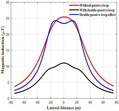
The evolution of the lateral magnetic field profile, including the one that considers the double passive compensation loop, is depicted in Figure 21, which shows the results obtained when the height from the surface is 1 meter. As can be seen in this figure, there is a pronounced decrease in the magnetic field value at all positions in the transmission line corridor, where the percentage of this reduction becomes as high as 56.5% from the original value of the magnetic field, which is at the center of the power line.
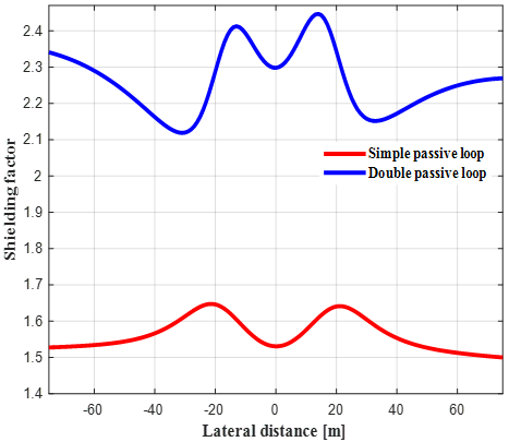
Figure 22 depicts the effectiveness of passive loops by presenting the magnetic reduction coefficient. It is evident that the presence of these passive loops under the conductors of the overhead power line generally reduces the magnetic field intensity symmetrically along the corridor of this power line. For a single passive loop, the magnetic attenuation coefficient is on average below the power line center, and then increases slowly with distance from this point, reaching a maximum value of 1.65, which corresponds to a maximum reduction rate of 40.64 %. From there, it gradually decreases towards both lateral sides. For a double passive loop, the coefficient increases considerably, reaching a maximum value of 2.45, which corresponds to a reduction rate of 60.34%. Consequently, it can be concluded that the double passive loop significantly reduces the magnetic field at every point along the power line corridor, more effectively than the single passive loop.
Figure 21. Magnetic induction profile at 1 m above ground level featuring a double passive loop configuration
Figure 22. Reduction factor for simple and double passive compensation loop
Figure 23. Magnetic induction profile at 1 m above the ground with simple passive loop using transmission line method
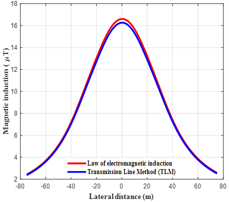
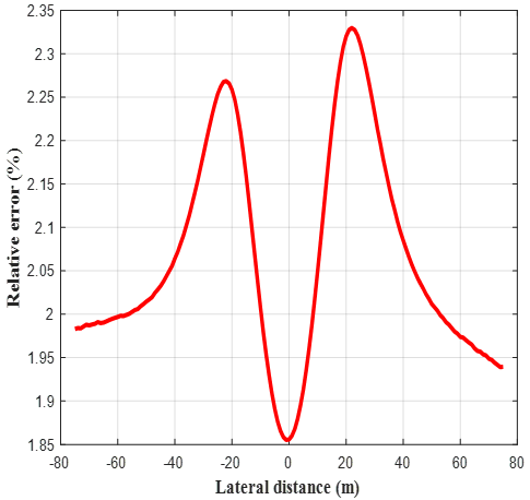
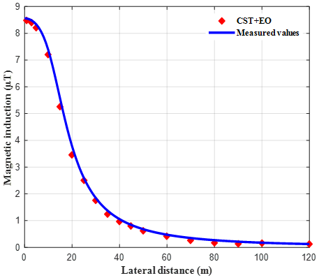
The final stage in the present case study involves testing the selected methodology by comparing the simulated results obtained from the use of this methodology with those derived using the multi-conductor transmission line technique. As shown in Figure 23, the graph for the magnetic field prior to the implementation of the simple passive loop and its compensation field is almost perfectly similar to that illustrated in Figure 19. To confirm accuracy, using the curves superposition, as Figure 24 shows, the graphs obtained for both methods are almost identical, depicting a perfect agreement with a very small margin of error. This comparison is clear and conclusive, thus confirming the validity of the proposed methodology. Figure 25 clearly shows how the relative error of the two methods is calculated, revealing that the maximum relative error is 2.33 %, a value well below the acceptable limit within the measurement range. This process confirms the results obtained and demonstrates the effectiveness of the adopted method. To confirm the accuracy of the proposed method, it was compared to magnetic induction measurement values reported in the literature for a similar geometric configuration [99], as shown in Figure 26. A slight difference was observed between the two values at 1 meter above the ground surface. Generally, the measured value is lower than the calculated value, mainly due to measurement conditions that are far from ideal, since the terrain is not flat and there are objects that act as shields, whereas the values calculated numerically under these conditions correspond to an ideal situation.
Figure 24. Comparison of magnetic induction values between the both simulations methods
Figure 25. Relative error values of the magnetic field obtained by the two calculation approaches
Figure 26. Comparison of the calculated and measured magnetic induction values mentioned in reference [99]
This study presents a robust quasi-static model combining the CST with the EO to obtain the optimal parameters defining the analysis and design process of passive compensation loops, thus ensuring highly accurate results. The results show that the magnetic field distribution is symmetric with respect to the power line center, reaching its maximum directly beneath the conductors and decreasing rapidly with lateral distance, and that the average value of the magnetic field, taking into account the conductor sag, is approximately equal to its value when it is neglected. The optimized configurations demonstrate that passive compensation loops are effective in reducing magnetic field exposure within the power transmission line corridor. In particular, the double passive loop provides superior performance, achieving a maximum reduction of 60.34% at 1 m above ground level, compared to 40.64% for the single passive loop. The obtained results are compared with those produced using a simulation based on the multi-conductor transmission line approach; A strong agreement was observed, with discrepancies not exceeding 2.33%, confirming the accuracy and reliability of the proposed CST-EO hybrid method. The proposed approach is applicable under quasi-static conditions, particularly for extremely low-frequency (ELF) UHV transmission lines operating at power industrial frequency, assuming steady-state current operation, with a uniform geometric configuration of overhead power conductors and flat terrain conditions.
The authors express gratitude to the Laboratory of Applied and Didactic Sciences at the Higher Normal School of Laghouat, the Electrical Engineering Department of the Faculty of Technology, and the Laboratory for Analysis and Control of Energy Systems and Electrical Systems (LACoSERE laboratory) at Ammar Telidji University of Laghouat, Algeria, for their support during this study. The authors would like to acknowledge the Deanship of Graduate Studies and Scientific Research, Taif University for funding this work.
[1] Mir, A.A., Alghassab, M., Ullah, K., Khan, Z.A., Lu, Y., Imran, M. (2020). A review of electricity demand forecasting in low and middle income countries: The demand determinants and horizons. Sustainability, 12(15): 5931. https://doi.org/10.3390/su12155931
[2] Rao, N.D. (2013). Does better electricity supply increase household enterprise income in India? Energy Policy, 57: 532-541. https://doi.org/10.1016/j.enpol.2013.02.025
[3] Liu, Z. (2015). Global energy development: The reality and challenges. In Global Energy Interconnection, Academic Press, pp. 1-64. https://doi.org/10.1016/B978-0-12-804405-6.00001-4
[4] Zainuddin, N.M., Rahman, M.A., Kadir, M.A., et al. (2020). Review of thermal stress and condition monitoring technologies for overhead transmission lines: Issues and challenges. IEEE Access, 8: 120053-120081. https://doi.org/10.1109/ACCESS.2020.3004578
[5] Simkó, M. (2008). Possible effects of electromagnetic fields (EMF) on human health—Opinion of the scientific committee on emerging and newly identified health risks (SCENIHR). Toxicology, 246(2-3): 248-250.
[6] Barnes, F., Freeman, J.E.R. (2022). Some thoughts on the possible health effects of electric and magnetic fields and exposure guidelines. Frontiers in Public Health, 10: 994758. https://doi.org/10.3389/fpubh.2022.994758
[7] Singh, S., Kapoor, N. (2014). Health implications of electromagnetic fields, mechanisms of action, and research needs. Advances in Biology: 198609. https://doi.org/10.1155/2014/198609
[8] Razek, A. (2022). Biological and medical disturbances due to exposure to fields emitted by electromagnetic energy devices—A review. Energies, 15(12): 4455. https://doi.org/10.3390/en15124455
[9] Anirudh Balaji. (2015). Effect of high voltage transmission lines on human, health, plant life, and animal activity. International Research Journal of Engineering and Technology, 2(3): 441-446.
[10] CIGRE, W. (1980). Electric and magnetic fields produced by transmission systems: Description of phenomena, practical guide for calculation. Paris.
[11] Tanaka, K., Mizuno, Y., Naito, K. (2010). Measurement of power frequency electric and magnetic fields nearby power facilities in several countries. In 9th International Symposium on EMC Joint with 20th International Wroclaw Symposium on EMC, EMC Europe, pp. 675-679. https://doi.org/10.23919/EMC.2010.10826291
[12] Gajšek, P., Ravazzani, P., Grellier, J., Samaras, T., Bakos, J., Thuróczy, G. (2016). Review of studies concerning electromagnetic field (EMF) exposure assessment in Europe: Low frequency fields (50 Hz–100 kHz). International Journal of Environmental Research and Public Health, 13(9): 875. https://doi.org/10.3390/ijerph13090875
[13] Fernie, K.J., Reynolds, S.J. (2005). The effects of electromagnetic fields from power lines on avian reproductive biology and physiology: A review. Journal of Toxicology and Environmental Health, Part B, 8(2): 127-140.
[14] Hardell, L., Sage, C. (2008). Biological effects from electromagnetic field exposure and public exposure standards. Biomedicine & Pharmacotherapy, 62(2): 104-109. https://doi.org/10.1016/j.biopha.2007.12.004
[15] Markov, M.S. (2013). Effects of electromagnetic fields on biological systems. Electromagnetic Biology and Medicine, 32(2): 121-122. https://doi.org/10.3109/15368378.2013.776333
[16] Duhaini, I. (2016). The effects of electromagnetic fields on human health. Physica Medica, 32: 213. https://doi.org/10.1016/j.ejmp.2016.07.720
[17] Budnik, K., Machczyński, W. (2006). Contribution to studies on calculation of the magnetic field under power lines. European Transactions on Electrical Power, 16(4): 345-364. https://doi.org/10.1002/etep.90
[18] Petrović, G., Kilić, T., Garma, T. (2013). Measurements and estimation of the extremely low frequency magnetic field of the overhead power lines. Elektronika ir Elektrotechnika, 19(7): 33-36. https://doi.org/10.5755/j01.eee.19.7.5159
[19] Brauer, H., Ziolkowski, M. (2006). Magnet shape optimization using adaptive simulated annealing. Facta Universitatis-Series: Electronics and Energetics, 19(2): 165-172.
[20] Sahbudin, R.K.Z., Fauzi, S.A., Hitam, S., Mokhtar, M. (2010). Investigation of electrical potential and electromagnetic field for overhead high voltage power lines in Malaysia. Journal of Applied Sciences, 10(22): 2862-2868. https://doi.org/10.3923/jas.2010.2862.2868
[21] International Commission on Non-Ionizing Radiation Protection. (2010). Guidelines for limiting exposure to time-varying electric and magnetic fields (1 Hz to 100 kHz). Health Physics, 99(6): 818-836. https://doi.org/10.1097/HP.0b013e3181f06c86
[22] Bailey, W.H., Bodemann, R., Bushberg, J., et al. (2019). Synopsis of IEEE Std C95.1™-2019 “IEEE standard for safety levels with respect to human exposure to electric, magnetic, and electromagnetic fields, 0 Hz to 300 GHz”. IEEE Access, 7: 171346-171356. https://doi.org/10.1109/ACCESS.2019.2954823
[23] Landini, M., Mazzanti, G., Mandrioli, R. (2021). Procedure for verifying population exposure limits to the magnetic field from double-circuit overhead power lines. Electricity, 2(3): 342-358. https://doi.org/10.3390/electricity2030021
[24] Stam, R. (2018). Comparison of international policies on electromagnetic fields: Power frequency and radiofrequency fields. National Institute for Public Health and the Environment.
[25] Sayed, A.R., Anis, H.I. (2018). Technical and economic feasibility of passive shielding used to mitigate power lines’ magnetic fields. WSEAS Transactions on Circuits and Systems, 17: 38-46.
[26] Ranković, A. (2017). Novel multi-objective optimization method of electric and magnetic field emissions from double-circuit overhead power line. International Transactions on Electrical Energy Systems, 27(2): e2243. https://doi.org/10.1002/etep.2243
[27] Jayalakshmi, N.Y., Deepa, S. (2016). Modelling of electric and magnetic fields under high voltage AC transmission line. IOSR Journal of Electrical and Electronics Engineering, 11(3): 24-31.
[28] Lee, B.Y., Myung, S.H., Ju, M.N., et al. (2014). Assessment of magnetic field mitigation and electrical environmental effects for commercially operating 154kV transmission lines with passive loop. Journal of Electrical Engineering & Technology, 9(3): 991-996. https://doi.org/10.5370/JEET.2014.9.3.991
[29] Said, I., Hussain, H., Kamaruddin, M. (2011). Magnetic field distribution due to shielding in a three-phase source. Journal of Applied Sciences, 11(7): 1351-1355.
[30] Canova, A., Giaccone, L., Cirimele, V. (2019). Active and passive shield for aerial power lines. In 25th International Conference on Electricity Distribution, Madrid, Spain, pp. 1-5.
[31] Salinas, E., Bottauscio, O., Chiampi, M., et al. (2009). Mitigation techniques of power frequency magnetic fields originated from electric power systems. Electra, 242: 75-83.
[32] Salinas, E. (2001). Mitigation of power-frequency magnetic fields with applications to substations and other parts of the electric network. Chalmers Tekniska Hogskola, Sweden.
[33] Cruz Romero, P., Izquierdo, C., Burgos, M., Ferrer, L.F., Soto, F., Llanos, C., Pacheco, J.D. (2002). Magnetic field mitigation in power lines with passive and active loops. In Proceedings of the CIGRE Session.
[34] Canova, A., Fabio, F., Giaccone, L., Guerrisi, A., Repetto, M. (2012). Magnetic field mitigation by means of passive loop: Technical optimization. COMPEL - The International Journal for Computation and Mathematics in Electrical and Electronic Engineering, 31(3): 870-880. https://doi.org/10.1108/03321641211209762
[35] Cruz, P., Izquierdo, C., Burgos, M. (2003). Optimum passive shields for mitigation of power lines magnetic field. IEEE Transactions on Power Delivery, 18(4): 1357-1362. https://doi.org/10.1109/TPWRD.2003.817754
[36] Bravo-Rodríguez, J.C., Del-Pino-López, J.C., Cruz-Romero, P. (2019). A survey on optimization techniques applied to magnetic field mitigation in power systems. Energies, 12(7): 1332. https://doi.org/10.3390/en12071332
[37] Książkiewicz, M. (2015). Passive loop coordinates optimization for mitigation of magnetic field value in the proximity of a power line. Computer Applications in Electrical Engineering, 13.
[38] Rebolini, M., Forteleoni, M., Capra, D. (2017). Passive cancellation loops: Case study, model simulation and field test on a real HV overhead line in Italy. In 2017 AEIT International Annual Conference, Cagliari, Italy, pp. 1-6. https://doi.org/10.23919/AEIT.2017.8240502
[39] Cruz, P., Riquelme, J.M., De La Villa, A., Martínez, J.L. (2007). GA-based passive loop optimization for magnetic field mitigation of transmission lines. Neurocomputing, 70(16-18): 2679-2686. https://doi.org/10.1016/j.neucom.2006.05.016
[40] Romero, P.C., Santos, J.R., Del Pino López, J.C., De La Villa Jaén, A., Ramos, J.L.M. (2007). A comparative analysis of passive loop-based magnetic field mitigation of overhead lines. IEEE Transactions on Power Delivery, 22(3): 1773-1781. https://doi.org/10.1109/TPWRD.2007.899784
[41] Budnik, K., Machczyński, W. (2013). Reduction of magnetic field from a power line using a passive loop conductor. Computer Applications in Electrical Engineering, 11: 46-63.
[42] Faria, J.B., Almeida, M. (2007). Accurate calculation of magnetic-field intensity due to overhead power lines with or without mitigation loops with or without capacitor compensation. IEEE Transactions on Power Delivery, 22(2): 951-959. https://doi.org/10.1109/TPWRD.2006.883025
[43] Faramarzi, A., Heidarinejad, M., Stephens, B., Mirjalili, S. (2020). Equilibrium optimizer: A novel optimization algorithm. Knowledge-Based Systems, 191: 105190. https://doi.org/10.1016/j.knosys.2019.105190
[44] Ghoneim, S.S. (2013). Charge and current simulation method with boundary element method for grounding system calculations in case of multi-layer soil. IOSR Journal of Engineering, 3(6): 14-22.
[45] Djekidel, R., Ahmed, B.S., Samar, A. (2019). Accurate computation of magnetic induction generated by HV overhead power lines. Facta Universitatis, Series: Electronics and Energetics, 32(2): 267-285. https://doi.org/10.2298/FUEE1902267R
[46] Abdel-Salam, M., Abdallah, H., El-Mohandes, M.T., El-Kishky, H. (1999). Calculation of magnetic fields from electric power transmission lines. Electric Power Systems Research, 49(2): 99-105. https://doi.org/10.1016/S0378-7796(98)00078-9
[47] Anany, A.A. (2021). Passive loop mathematical model as a reduction method for overhead line magnetic field. In IET Conference Proceedings, 2021(6): 1046-1050. https://doi.org/10.1049/icp.2021.1837
[48] Wall, C.A., Arnera, P.L., Barbieri, M.B. (2012). Implementation of a tool for magnetic field mitigation using passive loops. In 2012 Sixth IEEE/PES Transmission and Distribution: Latin America Conference and Exposition (T&D-LA), pp. 807-810. https://doi.org/10.1109/TDC-LA.2012.6319095
[49] Lings, R. (2005). Overview of transmission lines above 700 kV. In 2005 IEEE Power Engineering Society Inaugural Conference and Exposition in Africa, Durban, South Africa, pp. 807-810. https://doi.org/10.1109/PESAFR.2005.1611782
[50] Sirjani, R., Hassanpour, B. (2011). Technical and economic assessment of upgrading a double-circuit 63 kV to a single-circuit 230 kV transmission line in Iran. Australian Journal of Basic and Applied Sciences, 5(12): 2090-2097.
[51] Albizu Flórez, I., Mazón Sainz-Maza, A.J., Fernández Herrero, E. (2011). A method for the sag-tension calculation in electrical overhead lines. International Review of Electrical Engineering, 6(3).
[52] Crasson, M. (2003). 50-60 Hz electric and magnetic field effects on cognitive function in humans: A review. Radiation Protection Dosimetry, 106(4): 333-340. https://doi.org/10.1093/oxfordjournals.rpd.a006369
[53] Mujezinovic, A., Turajlic, E., Alihodzic, A., Dautbasic, N., Dedovic, M.M. (2022). Novel method for magnetic flux density estimation in the vicinity of multi-circuit overhead transmission lines. IEEE Access, 10: 18169-18181. https://doi.org/10.1109/ACCESS.2022.3149393
[54] Deltuva, R., Lukočius, R. (2020). Distribution of magnetic field in 400 kV double-circuit transmission lines. Applied Sciences, 10(9): 3266. https://doi.org/10.3390/app10093266
[55] Miyamoto, Y., Baba, Y., Nagaoka, N., Ametani, A. (2015). Numerical electromagnetic field analysis of high-frequency wave propagation on an overhead conductor. IEEE Transactions on Electromagnetic Compatibility, 57(3): 587-590. https://doi.org/10.1109/TEMC.2015.2402658
[56] Hossain, M.K., Tasnim, L. (2025). Analysis the impact of ground conductivity source current speed and source current rise time on peak induced voltage on overhead conductors. Discover Electronics, 2: 3. https://doi.org/10.1007/s44291-025-00044-3
[57] Chatzineofytou, E.G., Spantideas, S.T., Nikolopoulos, C.D., et al. (2019). Decoupling of ground plane effect on low frequency magnetic and electric field measurements & modeling. In 2019 ESA Workshop on Aerospace EMC (Aerospace EMC), Budapest, Hungary. https://doi.org/10.23919/AeroEMC.2019.8788906
[58] Saied, M.M. (2008). Assessment and optimal passive-loop mitigation of power lines’ magnetic fields. In 2008 Asia-Pacific Symposium on Electromagnetic Compatibility and 19th International Zurich Symposium on Electromagnetic Compatibility, Singapore, pp. 807-810. https://doi.org/10.1109/APEMC.2008.4559998
[59] Caparelli, E., Tomasi, D. (2001). Um cálculo analítico do campo magnético usando a lei de Biot Savart. Revista Brasileira de Ensino de Física, 23: 284-288. https://doi.org/10.1590/S1806-11172001000300005
[60] Yao, D., Li, B., Deng, J., Huang, D., Wu, X. (2008). Power frequency magnetic field of heavy current transmit electricity lines based on simulation current method. In 2008 World Automation Congress, Hawaii, USA, pp. 1-4.
[61] Radwan, R., Abdel-Salam, M., Mahdy, A.B., Samy, M. (2011). Laboratory validation of calculations of magnetic field mitigation underneath transmission lines using passive and active shield wires. Innovative Systems Design and Engineering, 2(4): 218-232.
[62] Djekidel, R., Bessedik, S.A. (2020). ASA algorithm combined with current simulation method (CSM) for the magnetic induction under HV power lines in 3D analysis model. Advanced Electromagnetics, 9(2): 7-18. https://doi.org/10.7716/aem.v9i2.1345
[63] Radwan, R.M., Abdel-Salam, M., Samy, M.M., Mahdy, A.M. (2015). Passive and active shielding of magnetic fields underneath overhead transmission lines theory versus experiment. In Proceedings of the 17th International Middle East Power Systems Conference, Mansoura, Egypt, pp. 1-10.
[64] Meriouma, T., Bessedik, S.A., Djekidel, R. (2021). Modelling of electric and magnetic field induction under overhead power line using improved simulation techniques. European Journal of Electrical Engineering, 23(4). https://doi.org/10.18280/ejee.230402
[65] Riba Ruiz, J.R., Garcia Espinosa, A. (2011). Magnetic field generated by sagging conductors of overhead power lines. Computer Applications in Engineering Education, 19(4): 787-794. https://doi.org/10.1002/cae.20365
[66] Filippopoulos, G., Tsanakas, D. (2005). Analytical calculation of the magnetic field produced by electric power lines. IEEE Transactions on Power Delivery, 20(2): 1474-1482. https://doi.org/10.1109/TPWRD.2004.839184
[67] Mamishev, A., Nevels, R., Russell, B. (2002). Effects of conductor sag on spatial distribution of power line magnetic field. IEEE Transactions on Power Delivery, 11(3): 1571-1576. https://doi.org/10.1109/61.517518
[68] Alihodzic, A., Mujezinovic, A., Turajlic, E., Dedovic, M.M. (2022). Determination of electric and magnetic field calculation uncertainty in the vicinity of overhead transmission lines. Journal of Microwaves, Optoelectronics and Electromagnetic Applications, 21: 392-413. https://doi.org/10.1590/2179-10742022v21i3262024
[69] Djekidel, R., Bessedik, S.A., Spiteri, P., Mahi, D. (2018). Passive mitigation for magnetic coupling between HV power line and aerial pipeline using PSO algorithms optimization. Electric Power Systems Research, 165: 18-26. https://doi.org/10.1016/j.epsr.2018.08.014
[70] Budnik, K., Machczyński, W. (2013). Power line magnetic field mitigation using a passive loop conductor. Poznan University of Technology Academic Journals. Electrical Engineering, 137-145.
[71] Houicher, S.E., Djekidel, R., Bessedik, S.A. (2025). Optimized passive and active shielding of magnetic induction generated by ultra-high-voltage overhead power lines. International Journal of Electrical and Computer Engineering, 15(6): 5144-5161. https://doi.org/10.11591/ijece.v15i6.pp5144-5161
[72] Dein, A.Z.E., Gouda, O.E., Lehtonen, M., Darwish, M.M.F. (2022). Mitigation of the electric and magnetic fields of 500-kV overhead transmission lines. IEEE Access, 10: 33900-33908. https://doi.org/10.1109/ACCESS.2022.3161932
[73] Marin, J.L.A., Villalobos, L.C., Vera-Dimas, J.G., Jaime, J.S., Saldarriaga-Noreña, H.A., Gutierrez, H.H. (2025). Mitigation of magnetic field levels in bipolar transmission lines of 500 and 600 kV in HVDC. Energies, 18: 5022. https://doi.org/10.3390/en18185022
[74] Ahmed, E.M., AbdElrazek, A.S., Alkhafa, A., Ibrahim, K.H. (2025). Mitigation of magnetic fields in overhead power lines through genetic algorithm-based electromechanical compensation. Journal of Magnetism and Magnetic Materials, 631: 173493. https://doi.org/10.1016/j.jmmm.2025.173493
[75] Alihodzic, A., Mujezinovic, A., Turajlic, E. (2021). Electric and magnetic field estimation under overhead transmission lines using artificial neural networks. IEEE Access, 9: 105876-105891. https://doi.org/10.1109/ACCESS.2021.3099760
[76] Yamazaki, K., Kawamoto, T., Fujinami, H. (2002). Requirements for power line magnetic field mitigation using a passive loop conductor. IEEE Transactions on Power Delivery, 15(2): 646-651. https://doi.org/10.1109/61.852999
[77] Kim, E.S. (2021). A study on magnetic field reduction design technique around 345 kV transmission line with 2-wire set passive loop. Journal of the Korean Society of Safety, 36(5): 10-17.
[78] Memari, A., Janischewskyj, W. (2002). Mitigation of magnetic field near power lines. IEEE Transactions on Power Delivery, 11(3): 1577-1586. https://doi.org/10.1109/61.517519
[79] Misakian, M. (2000). Equations for the magnetic field produced by one or more rectangular loops of wire in the same plane. Journal of Research of the National Institute of Standards and Technology, 105(4): 557. https://doi.org/10.6028/jres.105.045
[80] Buccella, C., Feliziani, M., Fuina, V. (2002). ELF magnetic field mitigation by active shielding. In ISIE 2002 - 2002 IEEE International Symposium on Industrial Electronics, L'Aquila, Italy, pp. 994-998. https://doi.org/10.1109/ISIE.2002.1025869
[81] Del Pino Lopez, J.C., Romero, P.C. (2010). The effectiveness of compensated passive loops for mitigating underground power cable magnetic fields. IEEE Transactions on Power Delivery, 26(2): 674-683. https://doi.org/10.1109/TPWRD.2009.2039150
[82] Ziolkowski, M., Gratkowski, S. (2009). Active, passive and dynamic shielding of static and low frequency magnetic fields. In VXV International Symposium on Theoretical Engineering, pp. 1-5.
[83] Falsaperla, R., Spagnoli, G., Rossi, P. (2006). Electromagnetic fields: Principles of exposure mitigation. International Journal of Occupational Safety and Ergonomics, 12(2): 195-200. https://doi.org/10.1080/10803548.2006.11076683
[84] Fu, Z., Hu, P., Li, W., Pan, J.S., Chu, S. (2021). Parallel equilibrium optimizer algorithm and its application in capacitated vehicle routing problem. Intelligent Automation and Soft Computing, 27(1): 233-247. https://doi.org/10.32604/iasc.2021.014192
[85] Lan, P., Hu, P., Li, W., Pan, J.S., Chu, S. (2021). An improved equilibrium optimizer algorithm and its application in LSTM neural network. Symmetry, 13(9): 1706.
[86] Guerraiche, K., Midouni, F., Sahraoui, N.E., Dekhici, L. (2023). Application of equilibrium optimizer algorithm for solving linear and non linear coordination of directional overcurrent relays. Advances in Electrical and Electronic Engineering, 20(4): 537-548. https://doi.org/10.15598/aeee.v20i4.4647
[87] Liu, Y., Ding, H., Wang, Z., Jin, G., Li, B., Yang, Z., Dhiman, G. (2023). A chaos-based adaptive equilibrium optimizer algorithm for solving global optimization problems. Mathematical Biosciences and Engineering, 20(9): 17242-17271. https://doi.org/10.3934/mbe.2023768
[88] Agnihotri, S., Atre, A., Verma, H. (2020). Equilibrium optimizer for solving economic dispatch problem. In 2020 IEEE 9th Power India International Conference, Sonepat, India, pp. 1-5. https://doi.org/10.1109/PIICON49524.2020.9113048
[89] Nguyen, T.A., Pham, D.C., Thanh, N.C., Nguyen, A.N. (2021). Implementation of equilibrium optimizer algorithm for MPPT in a wind turbine with PMSG. WSEAS Transactions on Systems and Control, 16: 216-223. https://doi.org/10.37394/23203.2021.16.18
[90] Djekidel, R., Bessedik, S.A. (2016). Estimation and mitigation of electrostatic interferences on metallic pipeline by HV overhead power line using differential evolution algorithm. Electrotehnica, Electronica, Automatica, 64(3).
[91] Peres, P.L., De Souza, C.R., Bonatti, I.S. (2003). ABCD matrix: A unique tool for linear two-wire transmission line modelling. International Journal of Electrical Engineering Education, 40(3): 220-229. https://doi.org/10.7227/IJEEE.40.3.5
[92] Deniz, E., Rashid, A., Hasan, O., Tahar, S. (2024). Formal verification of ABCD parameters based models for transmission lines. In International Symposium on Symbolic Computation in Software Science, pp. 20-37. https://doi.org/10.1007/978-3-031-69042-6_2
[93] Kim, D. (2022). ABCD parameters in series-series compensation wireless power transfer system. In 2022 IEEE Sustainable Power and Energy Conference (iSPEC), Perth, Australia. https://doi.org/10.1109/iSPEC54162.2022.10033072
[94] Kryukov, A., Suslov, K., Van Thao, L., Hung, T.D., Akhmetshin, A. (2022). Power flow modeling of multi-circuit transmission lines. Energies, 15(21): 8249. https://doi.org/10.3390/en15218249
[95] Abdel-Salam, M., Al-Shehri, A. (2002). Induced voltages on fence wires and pipelines by AC power transmission lines. IEEE Transactions on Industry Applications, 30(2): 341-349. https://doi.org/10.1109/28.287525
[96] Djogo, G., Salama, M. (1997). Calculation of inductive coupling from power lines to multiple pipelines and buried conductors. Electric Power Systems Research, 41(1): 75-84. https://doi.org/10.1016/S0378-7796(96)01162-5
[97] Micu, D.D., Christoforidis, G.C., Czumbil, L. (2013). AC interference on pipelines due to double circuit power lines: A detailed study. Electric Power Systems Research, 103: 1-8. https://doi.org/10.1016/j.epsr.2013.04.008
[98] Xu, Z., Dong, H., Huang, H. (2015). Debates on ultra-high-voltage synchronous power grid: The future super grid in China? IET Generation, Transmission & Distribution, 9: 740-747. https://doi.org/10.1049/iet-gtd.2014.0281
[99] Vujević, S., Lovrić, D., Modrić, T. (2011). 2D computation and measurement of electric and magnetic fields of overhead electric power lines. In Proceedings of the Joint INDS'11 & ISTET'11, Klagenfurt am Wörthersee, Austria, pp. 1-6. https://doi.org/10.1109/INDS.2011.602479