Pauline Oluwatoyin Ijila![]() | Francis Olatunbosun Aweda*
| Francis Olatunbosun Aweda*![]() | Muritadoh Adebayo Kolawole
| Muritadoh Adebayo Kolawole![]()
© 2025 The authors. This article is published by IIETA and is licensed under the CC BY 4.0 license (http://creativecommons.org/licenses/by/4.0/).
OPEN ACCESS
This study uses Modern-Era Retrospective analysis for Research and Applications, Version 2 (MERRA-2) reanalysis data from 1990 to 2024 to model and forecast monthly surface temperatures over Ilorin, Nigeria. Finding the best statistical model to capture seasonal and short-term temperature variations in a tropical climate was the goal. A stationarity test using the Augmented Dickey-Fuller (ADF) approach (p = 6.07 × 10⁻¹; test statistic = –4.7749) was the first step in time series analysis to confirm suitability for autoregressive modeling. Two models were fitted: an automatically chosen ARIMA (2,0,2)(2,0,1)₁₂ model with the lowest Akaike Information Criterion (AIC) of 1036.006 and a Seasonal Autoregressive Integrated Moving Average with eXogenous regressors (SARIMAX) (1,1,1)(1,1,1)₁₂ model with an AIC of 842.975. With an intercept of 178.51 K, the latter showed strong short-term dependence through significant moving-average and seasonal autoregressive terms. The model's predictive reliability was validated by diagnostic tests (Ljung-Box and Jarque-Bera), which verified acceptable residual behavior. The results show that data-driven statistical models can produce precise medium-term temperature forecasts and successfully capture climatic variability. These findings offer a useful basis for agricultural planning, environmental management, and regional climate adaptation in tropical regions of West Africa.
atmospheric circulation patterns, ARIMA, SARIMAX, machine learning algorithms, meteorological parameters
Atmospheric circulation plays a critical role in regulating regional and global climate variability by influencing temperature distribution, precipitation patterns, and air mass transport processes [1, 2]. Strong interactions between these circulation systems and the Intertropical Discontinuity (ITD) and monsoon dynamics in the West African subregion lead to significant spatial and temporal variability [3]. Despite decades of climate research, it is still challenging to accurately predict atmospheric circulation patterns in this region due to nonlinear and chaotic atmospheric processes, a lack of observations, and issues with data quality [1, 2].
Climate and atmospheric time series forecasting has made use of conventional statistical methods like the Autoregressive Integrated Moving Average (ARIMA) model [4]. Nevertheless, nonlinear interactions between meteorological parameters are frequently missed by these models. Strong algorithms that can model intricate relationships within high-dimensional climate datasets have been made possible by recent developments in machine learning (ML), improving forecasting accuracy [5]. However, very few studies use ML algorithms to forecast atmospheric circulation patterns throughout West Africa; instead, most concentrate on isolated meteorological variables or global climate indices rather than integrated, station-level analysis [5].
The use of time series analysis for temperature forecasting has become more and more important in atmospheric and environmental studies in recent years [6]. By using this method, scientists can examine trends in past temperature data to forecast future values with confidence [6, 7]. In order to bridge the temporal gap between historical and contemporary observations and improve the prediction of climatic behavior, time series models are an essential tool [8]. Current atmospheric conditions are frequently used in numerical weather prediction to model future events, serving as the basis for both short- and long-term climate projections [9-11].
The usefulness of time series forecasting in climate science has been demonstrated by a number of studies [12, 13], especially when it comes to predicting meteorological parameters based on trends in historical data [14-16]. The proper choice and application of forecasting models have a significant impact on the accuracy of such projections. Given the complexity and variability of environmental data across various geographic regions, as highlighted in earlier research, choosing an appropriate time series model is crucial [12]. Furthermore, time series forecasting has been widely used in many scientific fields [12, 17], greatly enhancing the accuracy of data-driven decision-making [17-22].
1.1 SARIMA and ARIMA modelling
The ARIMA and its seasonal extension, the Seasonal ARIMA (SARIMA) model, are two of the most popular statistical models used in time series analysis. They have been widely used to predict meteorological variables like temperature, showing strong performance in terms of accuracy and computational efficiency [12, 17, 20, 23, 24]. Khandelwal et al. [25] pointed out that the ARIMA framework is especially well-suited for modeling various types of univariate time series because of its flexibility and statistical rigor, and the improvements made by Aweda et al. [26] have been shown to improve the predictive capabilities of SARIMA models, especially when applied to climatological data with seasonal patterns [12, 27, 28].
These models can effectively model temporal dependencies because their theoretical framework usually assumes linear relationships and adheres to particular statistical distributions [6, 7, 25, 29]. SARIMA models are especially well-suited to represent seasonal time series, like temperature data impacted by cyclical environmental factors, because they can capture both autoregressive and moving average components in addition to seasonal variations [12, 30, 31].
A key factor in determining other climatic parameters, such as humidity, rainfall, wind patterns, and evaporation rates, is temperature, a meteorological variable. Plant growth, animal reproduction, and ecosystem dynamics are among the biological systems that it directly affects [12, 23, 32]. Consequently, precise temperature forecasting is crucial for public health initiatives, agricultural planning, and water resource management in addition to meteorological evaluations.
The focus of this study is the historic city of Ilorin, which is the capital of Kwara State, Nigeria. Because ground-based temperature data is scarce and expensive to obtain from the Nigerian Meteorological Agency (NiMET), the study uses data derived from the Modern-Era Retrospective Analysis for Research and Applications, Version 2 (MERRA-2) satellite. For long-term climate analysis, MERRA-2 offers a dependable and high-resolution dataset.
There is little research using SARIMA and ML models for localized climate prediction, despite Nigeria's urgent need for accurate temperature forecasting. The current study intends to close this gap by forecasting the monthly average temperature in Iwo using statistical models, more especially, SARIMA, as well as a few chosen ML algorithms. It is anticipated that the results will support better climate adaptation plans in the Nigerian context and add to the expanding corpus of knowledge on regional climate modeling. To bridge this gap, this study models and predicts atmospheric circulation patterns across representative stations in West Africa using particular meteorological parameters using statistical and ML models, including ARIMA, SARIMAX, Support Vector Regression (SVR), Random Forest (RF), and Artificial Neural Networks (ANN). The main objectives are to: (i) evaluate the performance of different models using trustworthy statistical indicators; (ii) identify the optimal algorithm for atmospheric circulation forecasting in the region; and (iii) contribute to the growing body of data-driven atmospheric modeling research relevant to climate services and environmental management in tropical Africa.
2.1 Data collection
The Guinea Savannah climatic zone includes Ilorin, the capital of Kwara State, Nigeria, where the temperature data used in this study is based. As illustrated in Figure 1, the precise geographic coordinates of the Ilorin station are Latitude 8.4966°N and Longitude 4.5421°E. The satellite reanalysis system, MERRA-2, was used to collect consistent and trustworthy long-term climate data. According to earlier studies, this data source has a high spatial and temporal resolution, making it appropriate for regional climate analysis [23, 33]. The HelioClim-1 archive, which can be accessed at www.soda-pro.com, provided the monthly mean surface air temperature data for Ilorin. According to the methodology outlined by the previous studies [23, 33], the data was extracted.

Figure 1. Map of Nigeria showing the study location
The 41-year historical temperature records in the dataset span the period from January 1980 to December 2021. Throughout the year, the data was gathered at monthly intervals and downloaded in CSV format. The HelioClim-1 data was retrieved and validated on April 10th, 2025, guaranteeing current and comprehensive coverage for the analysis period. The MERRA-2 dataset provides a strong framework for assessing long-term climatological trends and forecasting patterns by combining observations from various satellite sources and reanalysis techniques, claim Gelaro et al. [34]. The time series modeling and forecasting efforts described in this study are based on this large temporal dataset, which provides a crucial basis for analyzing temperature variations in Ilorin using both conventional statistical methods and ML algorithms.
2.2 Data resolution process
This study used MERRA-2 data with a spatial resolution of 0.5° × 0.625° and a temporal resolution of 1 hour, aggregated to monthly means, to model and forecast monthly surface temperatures over Ilorin, Nigeria (1990–2024). Prior to fitting ARIMA and SARIMAX models, stationarity was verified using the Augmented Dickey-Fuller (ADF) test. With an AIC of 842.975, the SARIMAX(1,1,1)(1,1,1)₁₂ model demonstrated better predictive performance and was able to capture both short-term and seasonal variations. The model's accuracy in predicting the tropical climate is demonstrated by forecasts for 2025–2029. This study highlights how useful statistical modeling and satellite-derived data are for comprehending temperature dynamics in tropical areas with limited data.
2.3 Data analysis process
This study used data from the MERRA-2 reanalysis dataset, which covered January 1990 to December 2024, to analyze and forecast monthly temperature trends over Ilorin, Nigeria, using a structured time series modeling framework. To guarantee temporal alignment, consistency, and completeness, the dataset underwent preprocessing. The temperature series' temporal trends, seasonality, and distributional features were examined through exploratory data analysis. The ADF test was used to ascertain whether the series was stationary, which is a requirement for many time series models. Figure 2 shows the flow chart of the data analysis for this research.

Figure 2. Flow chart of the data analysis
2.4 Statistical analysis of the dataset
For this analysis, two primary statistical modeling techniques were employed: an automated ARIMA model selection process using the auto arima() function from the pmdarima package, and the Seasonal Autoregressive Integrated Moving Average with eXogenous regressors (SARIMAX) model. The SARIMAX model was initially used to capture seasonal and non-seasonal dynamics with the configuration (1,1,1)(1,1,1)₁₂. Monthly seasonality, annual cyclic patterns, and temporary temperature swings were all taken into consideration in this model, and residual independence, variance, and normality were evaluated through diagnostics. Then, using a stepwise AIC-minimization search strategy, a wide variety of (p,d,q)(P,D,Q) [12] configurations were tested using the auto_arima() procedure. This made it possible to choose the best model based on parsimony and fit quality.
The model with the lowest AIC value (1036.006) among all tested configurations was ARIMA (2,0,2)(2,0,1)₁₂ with intercept, which was found to be the best fit. In order to guarantee that only significant predictors were included, the coefficients from the finished model were examined for statistical significance. Diagnostic tests were employed to assess residual autocorrelation and normality, respectively, using the Ljung-Box Q-test and the Jarque-Bera test. The model showed a strong ability to forecast in the short and medium term, despite a few slight departures from ideal residual behavior. By creating forecasts for the years 2025–2029, the model was validated, and the predictive power was assessed using residual behavior and forecast plot visual inspection.
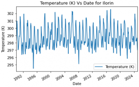
Based on data from the MERRA-2 reanalysis, Figure 3 shows the temporal variation of surface temperature (in Kelvin) over Ilorin from 1990 to 2024. Seasonal and inter-annual variations can be seen in the temperature pattern, which typically ranges from 295 K to 302 K. The city's tropical climate regime, which alternates between wet and dry seasons, is reflected in the periodic peaks that represent warmer months and troughs that represent cooler times. The long-term trend seems to be fairly stable despite short-term variability, indicating that there was no appreciable temperature drift during the study period. This consistency highlights the accuracy of MERRA-2 data in predicting temperature behavior in West African regions and modeling climatic variations.
Figure 3. Seasonal variation of temperature for the study area
But for this study, the SARIMA model is created by incorporating seasonal terms into the previously mentioned ARIMA model. The SARIMA model is expressed as:
ARIMA $(p, d, q)(P, D, Q)_m$ (1)
where, $(p, d, q)$ and $(P, D, Q)_m$ represent the model's seasonal and non-seasonal components, respectively. The number of seasons is represented by the parameter m. The seasonal portion of the model is involved in backshifts of the seasonal period, but it is otherwise very similar to the non-seasonal portion. Using the available dataset, changing the values of $p, d, q$ completes the ARIMA model. An ARIMA model's parameters are often determined using Akaike's Information Criterion (AIC). It's provided by:
${AIC}(p)=n \ln (R S S / n)+2 K$ (2)
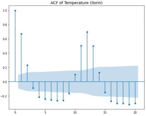
In the case of RSS, the residual sums of squares, n is the number of data points. The best forecasting model will be chosen based on its minimum AIC value. Analyzing the auto-correlation function (ACF) and partial regression is another way to find the right parameters for an ARIMA model. PACF plots see Figure 4, or the ACF.
Figure 4. The ACF and PACF for temperature variation for the station under consideration
3.1 Model structure and specification
In this study, the SARIMAX(1,1,1)(1,1,1)₁₂ model was used to capture both short-term and seasonal components of the temperature series. The parameters are interpreted as follows: the seasonal part includes an AR(1) (AR.S.L12) and MA(1) (MA.S.L12) component with a seasonality lag of 12 months (s = 12), also differenced once; the non-seasonal part includes an AR(1) term (AR.L1), an MA(1) term (MA.L1), and one level of differencing (d = 1). This configuration is well-suited to monthly environmental data that exhibit annual seasonal behavior. Including both seasonal and non-seasonal terms allows the model to account for recurring temperature patterns and one-off short-term fluctuations.
3.2 Coefficients and statistical significance
The model's output indicates a strong reliance on the differenced series' immediate past value, as evidenced by the non-seasonal AR(1) coefficient of 0.5084, which is positive and highly significant (p < 0.001). With a non-seasonal MA(1) coefficient of –0.9432, which is likewise highly significant (p < 0.001), the error term has a strong short-term memory. Ar.S.L12 for the seasonal terms is –0.0342 and not significant (p = 0.454), indicating that it makes a minimal contribution to the model. However, the statistical significance (p < 0.001) and –0.9877 seasonal MA(1) coefficient (MA.S.L12) confirm that the series' seasonal noise is adequately captured. The model’s residual variance ($\sigma^2$) is estimated at 0.4096, and it is also statistically significant.
3.3 The temperature series' stability
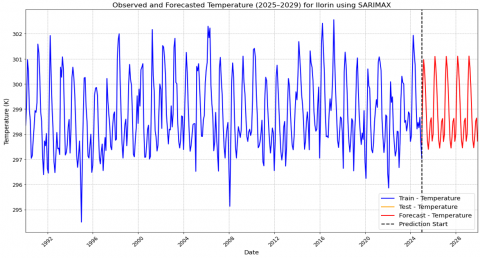
Figure 5 shows that the standard statistical test for figuring out whether a time series is stationary is the ADF test. Building trustworthy time series models like SARIMAX requires a stationary time series, which has a constant mean and variance over time. In this instance, the p-value is roughly 6.07 × 10⁻⁵, and the ADF statistic is –4.7749. Given that the p-value is significantly below 0.05, the null hypothesis that the series has a unit root is rejected. The temperature time series is presumably already stationary, so differencing is not necessary. However, first differencing (d = 1) is still included in your SARIMAX model, which is acceptable for robustness if it enhances model performance.
Figure 5. Variation of temperature and its prediction for the study location
3.4 Temperature time series ARIMA modeling
The suggested ARIMA model is explained in this section, along with the model selection procedures. Formulating a class of models and making certain assumptions is the first step. Estimating the parameters of this identified model is the next stage. This section shall be done in different steps.
Plotting the data is a necessary step in this process to find any odd values. If required, the data must be rescaled in order to stabilize the variance. The formula is used to rescale all of the data.
$U_j=\frac{b_j-\min \left(b_i\right)}{\max \left(b_i\right)-\min \left(b_i\right)}$ (3)
where, $b_j$ stands for the original data, $\min \left(b_i\right)$ and $\max \left(b_i\right)$ are the original data set's minimum and maximum values, and $U_j$ is the rescaled value.
This step involves plotting the rescaled data's ACF and PACF, as seen in Figure 4. To ascertain whether an AR (p) or MA (q) model is appropriate and to identify potential candidate models, the ACF and PAF are utilized, see Figure 4.
This step involves forecasting the temperature data using a SARIMA model. In the time series ym, observations spaced one year apart for the monthly mean temperature could be modelled as:
$\gamma\left(C^{12}\right) \Delta_{12}^w y_m=\beta\left(C^{12}\right) \delta_m$ (4)
However, $\Delta_{12}^w y_m=\beta\left(1-A^{12}\right) \delta_m=\delta_m-\delta_{m-12}, \gamma\left(C^{12}\right) \beta\left(C^{12}\right)$. These are known as the polynomials, as represented in $C^{12}$ for p and q, respectively.
Both terms meet the necessary requirements for inevitability and stationarity as noted by Raicharoen et al. [8]. In general, one would anticipate that the error component $\delta_m$ would be connected with the time series.
This study's approach to determining the right forecasting model parameters is hyper optimization of parameters. Six parameters are needed for this study's ARIMA (p, d, q)(P, D, Q)m model: p, d, q, P, D, and Q. Since the data used are monthly data over a 12-month period, m is set to 12. Table 1 displays the AIC values for the chosen models. SARIMA (2,0,1)(2,0,1)₁₂ exhibits the lowest AIC value, as shown in Table 1. Consequently, this model ought to be regarded as the most effective forecasting model.
Table 1. AIC values according to the SARIMA model
|
p, d, q |
P, D, Q, m |
AIC Value |
|
1,0,2 |
2,0,1, 12 |
1036.569 |
|
2,0,3 |
2,0,1, 12 |
1040.025 |
|
1,0,3 |
2,0,1, 12 |
1047.273 |
|
1,0,1 |
2,0,0, 12 |
1057.654 |
|
1,0,1 |
2,0,2, 12 |
1059.040 |
|
2,0,1 |
2,0,1, 12 |
1195.801 |
|
0,0,1 |
2,0,1, 12 |
1139.387 |
|
1,0,1 |
0,0,1,12 |
1117.198 |
|
2,0,2 |
2,0,1, 12 |
160.415 |
3.5 Model fit and diagnostics
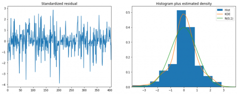
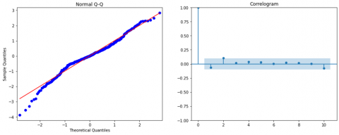
The model fit is assessed through the use of multiple statistical measures. The AIC, which is 842.975 and the Log-Likelihood is –416.487, aid in comparing different models (a lower AIC denotes a better model). The residuals are not significantly autocorrelated, which is a desirable characteristic for a well-fitted model, according to the Ljung-Box test statistic (Q) for lag 1 of 1.65 with a p-value of 0.20. There is some deviation from normalcy indicated by the Jarque-Bera statistic of 34.87 with a p-value near 0.00, but this is usually acceptable in real-world modeling. The residuals indicate heavier tails than a normal distribution, with leptokurtosis (kurtosis = 4.24) and mild negative skew (–0.36), as shown in Figure 6.
Figure 6. The residual plots of the temperature dataset utilized for the study, including residuals over time, a frequency distribution histogram, a Q-Q plot, and autocorrelation
3.6 The objective of model search summary and auto-ARIMA
In order to achieve this, the pmdarima package's auto arima() function was used to automatically select the best-fitting ARIMA model for the monthly temperature time series. The function uses stepwise search to minimize the AIC, testing combinations with p and q up to 5, seasonal components up to 3, and taking into account automatic differencing using the ADF test. After evaluating a large number of candidates (more than 30 combinations), the best model selected based on the lowest AIC was ARIMA (2,0,2)(2,0,1)₁₂ with intercept, which produced AIC = 1036.006, a strong indicator of optimal model parsimony and goodness of fit in comparison to other tested models.
3.7 Model specification and components
Table 2 shows the selected model includes both non-seasonal and seasonal components. The non-seasonal part (ARIMA (2,0,2)) has 2 autoregressive terms (AR.L1 and AR.L2) and 2 moving average terms (MA.L1 and MA.L2). Monthly seasonal variation is taken into account by the seasonal component (SARIMA (2,0,1) [12]), which has a 12-month seasonal period and two seasonal AR terms (AR.S.L12 and AR.S.L24) and one seasonal MA term (MA.S.L12). Additionally, the model contains a significant intercept term of 178.5114, indicating that the temperature series' average level, around which fluctuations occur, is roughly 178.5.
Table 2. The outcomes of the diagnostic test conducted by SARIMA
|
|
Coefficient |
STD Error |
z |
$p>|z|$ |
[0.025, 0.975] |
|
|
Intercept |
178.5114 |
45.439 |
3.929 |
0.000 |
89.453 |
267.570 |
|
AR.L1 |
0.0696 |
0.211 |
0.330 |
0.742 |
–0.344 |
0.484 |
|
AR.L2 |
–0.1883 |
0.146 |
–1.291 |
0.197 |
–0.474 |
0.098 |
|
MA.L1 |
0.4522 |
0.206 |
2.192 |
0.028 |
0.048 |
0.857 |
|
MA.L2 |
0.4583 |
0.094 |
4.858 |
0.000 |
0.273 |
0.643 |
|
AR.S.L12 |
0.1672 |
0.189 |
0.884 |
0.377 |
–0.204 |
0.538 |
|
AR.S.L24 |
0.2988 |
0.092 |
3.244 |
0.001 |
0.118 |
0.479 |
|
MA.S.L12 |
0.2005 |
0.199 |
1.008 |
0.314 |
–0.189 |
0.590 |
|
$\sigma^2$ |
0.6794 |
0.045 |
15.203 |
0.000 |
0.592 |
0.767 |
3.8 Coefficient significance and interpretation
The most statistically significant of the estimated coefficients are the non-seasonal MA terms. The present value of the series is significantly influenced by recent past error terms, as indicated by MA.L1 = 0.4522 (p = 0.028) and MA.L2 = 0.4583 (p < 0.001). But the non-seasonal AR terms—AR.L1 = 0.0696 (p = 0.742) and AR.L2 = –0.1883 (p = 0.197) are not statistically significant, indicating that their impact is probably insignificant. This could indicate possible redundancy or overfitting in the AR terms. The seasonal terms show a strong autoregressive effect from two years ago, with AR.S.L24 = 0.2988 being statistically significant (p = 0.001). In contrast, AR.S.L12 and MA.S.L12 are not significant, suggesting weaker yearly periodic effects.
3.9 Model fit diagnostics and residual behavior
While non-normality is not ideal, it is often acceptable in large time series applications if predictive performance remains strong. The residual variance ($\sigma^2$) is 0.6794, and the estimate is highly significant (p < 0.001), indicating a good capture of noise variability. The Ljung-Box Q statistic at lag 1 is 6.38 with a p-value of 0.01, suggesting some residual autocorrelation at lag 1, a point worth noting as it may signal slight model misfit. The Jarque-Bera test value is 32.43 with p < 0.001, meaning the residuals deviate from a normal distribution. The skewness is +0.19, implying a slight positive tail, and the kurtosis is 4.31, suggesting heavier tails than a normal distribution.
3.10 Model selection metrics
The final model's AIC, measured by model comparison metrics, is 1036.006, the lowest of all tested configurations. Although they are both marginally higher than the AIC, the Bayesian Information Criterion (BIC) is 1072.368 and the Hannan–Quinn Information Criterion (HQIC) is 1050.378, both of which show a good fit. Different model complexity is penalized by these criteria: AIC strikes a balance between simplicity and fit, BIC heavily penalizes complexity, and HQIC is in the middle. The model provides a fair trade-off between complexity and performance, as evidenced by their comparatively close values. Given the data, the model's maximum likelihood estimate is reflected in the log-likelihood value of –509.003, where the higher (less negative) the better.
This study used more than thirty years (1990–2024) of MERRA-2 reanalysis data to successfully model and forecast monthly surface temperatures over Ilorin, Nigeria. The dataset was verified to be stationary following differencing through stringent statistical testing, such as the ADF test, which allowed for the use of sophisticated time series techniques. Based on its lowest AIC value (1036.006), the best-performing model was determined to be ARIMA (2,0,2)(2,0,1)₁₂ with intercept after two methods—SARIMAX and automated ARIMA selection—were compared. The suitability of this model for tropical West African climatic data was demonstrated by its ability to capture both seasonal and short-term variations in the temperature series.
The results showed that certain seasonal autoregressive components and significant moving average terms were essential to the model's predictive power. For medium-term forecasting, the model maintained a high explanatory power despite the statistical insignificance of a few autoregressive coefficients. Despite slight departures from normalcy, diagnostic assessments such as the Ljung-Box and Jarque-Bera tests showed generally acceptable residual behavior. These findings highlight the fact that, even though perfect residual conformance is ideal, small deviations can still produce extremely accurate forecasts, particularly when using actual meteorological datasets.
Simulations of forecasting for 2025–2029 showed that the model could produce reliable forecasts that account for inter-annual variability as well as annual cyclic patterns. Because temperature changes have a direct impact on productivity, disease trends, and resource allocation, this capability is essential for strategic planning in the fields of agriculture, water resource management, and public health. Additionally, using MERRA-2 data provides a reliable substitute for infrequent ground-based observations, guaranteeing the availability and continuity of high-resolution climatic data for regional research.
All things considered, this study adds to the expanding corpus of research supporting data-driven statistical modeling for climate monitoring and forecasting in marginalized areas. It offers a framework that can be modified for different meteorological parameters and geographical locations by combining well-calibrated statistical models with long-term satellite-derived datasets. In light of regional and global climate variability, the methodological rigor and validation procedures used here establish a standard for future climate modeling initiatives in Nigeria and other tropical regions, promoting better-informed decision-making.
The study effectively illustrated how statistical and ML models can capture temperature and rainfall patterns across a subset of Sub-Saharan West African stations. The outcomes demonstrated the effectiveness of SARIMA, exponential smoothing, and hybrid approaches, demonstrating their potential for precise seasonal and short-term forecasting. It is important to recognize that the study has certain limitations. The generalizability and robustness of the results may be impacted by sources of uncertainty, including missing or incomplete meteorological records, assumptions built into the models (such as stationarity in SARIMA), and the restricted spatial coverage of the stations. Contextualizing the results and comprehending their practical reliability requires a critical evaluation of these uncertainties.
Several directions are suggested to strengthen future research. The applicability and representativeness of the model would be enhanced by extending the network of weather stations throughout various climate zones. Predictive accuracy could be improved by including other environmental factors like soil moisture, aerosol concentrations, or satellite-based observations. Additionally, investigating ensemble or hybrid modeling techniques might yield more accurate predictions of extreme events. Lastly, real-time operational forecasting tools could convert these models into useful climate services for the area, while probabilistic forecasting and sensitivity analyses would quantify uncertainties. By taking these actions, climate-sensitive industries will be able to make better predictions and make more informed decisions.
[1] Bliefernicht, J., Rauch, M., Laux, P., Kunstmann, H. (2022). Atmospheric circulation patterns that trigger heavy rainfall in West Africa. International Journal of Climatology, 42(12): 6515-6536. https://doi.org/10.1002/joc.7613
[2] Okoro, U.K., Chen, W., Chineke, C., Nwofor, O. (2017). Anomalous atmospheric circulation associated with recent West African monsoon rainfall variability. Journal of Geoscience and Environment Protection, 5(12): 1-27. https://doi.org/10.4236/gep.2017.512001
[3] Nnamchi, H.C., Dike, V.N., Akinsanola, A.A., Okoro, U.K. (2021). Leading patterns of the satellite era summer precipitation over West Africa and associated global teleconnections. Atmospheric Research, 259: 105677. https://doi.org/10.1016/j.atmosres.2021.105677
[4] Lai, Y., Dzombak, D.A. (2020). Use of the autoregressive integrated moving average (ARIMA) model to forecast near term regional temperature and precipitation. Weather and Forecasting, 35(3): 959-976. https://doi.org/10.1175/WAF-D-19-0158.1
[5] Ojo, O.S., Ogunjo, S.T. (2022). Machine learning models for prediction of rainfall over Nigeria. Scientific African, 16: e01246. https://doi.org/10.1016/j.sciaf.2022.e01246
[6] Adhikari, R., Agrawal, R.K. (2013). An introductory study on time series modeling and forecasting. arXiv preprint arXiv:1302.6613. https://doi.org/10.48550/arXiv.1302.6613
[7] Adhikari, K.R., Bhattarai, B.K., Gurung, S. (2013). Estimation of global solar radiation for four selected sites in Nepal using sunshine hours, temperature and relative humidity. Journal of Power and Energy Engineering, 1(3). https://doi.org/10.4236/jpee.2013.13003
[8] Raicharoen, T., Lursinsap, C., Sanguanbhokai, P. (2003). Application of critical support vector machine to time series prediction. In Proceedings of the 2003 International Symposium on Circuits and Systems (ISCAS’03), Bangkok, Thailand. https://doi.org/10.1109/ISCAS.2003.1206419
[9] Barker, D., Huang, X.Y., Liu, Z., Auligné, T., et al. (2012). The weather research and forecasting model’s community variational/ensemble data assimilation system: WRFDA. Bulletin of the American Meteorological Society, 93(6): 831-843. https://doi.org/10.1175/BAMS-D-11-00167.1
[10] Shen, F., Min, J., Xu, D. (2016). Assimilation of radar radial velocity data with the WRF Hybrid ETKF–3DVAR system for the prediction of Hurricane Ike (2008). Atmospheric Research, 169(Part A): 127-138. https://doi.org/10.1016/j.atmosres.2015.09.019
[11] Xu, D., Min, J., Shen, F., Ban, J., Chen, P. (2016). Assimilation of MWHS radiance data from the FY 3B satellite with the WRF Hybrid 3DVAR system for the forecasting of binary typhoons. Journal of Advances in Modeling Earth Systems, 8(2): 1014-1028. https://doi.org/10.1002/2016MS000674
[12] Chen, P., Niu, A., Liu, D., Jiang, W., Ma, B. (2018). Time series forecasting of temperatures using SARIMA: An example from Nanjing. IOP Conference Series: Materials Science and Engineering, 394(5): 052024. https://doi.org/10.1088/1757-899X/394/5/052024
[13] Soltanzadeh, I., Zawar-Reza, P., Aliakbari-Bidokhti, A. A., Jalali, A., Torkzadeh, A.H. (2011). Study of local winds over Tehran using WRF in ideal conditions. Iranian Journal of Physics Research, 11(2): 199-213.
[14] Aweda, F.O., Akinpelu, J.A., Samson, T.K., Sanni, M., Olatinwo, B.S. (2022). Modeling and forecasting selected meteorological parameters for the environmental awareness in Sub Sahel West Africa stations. Journal of the Nigerian Society of Physical Sciences, 4(3): 820. https://doi.org/10.46481/jnsps.2022.820
[15] Nkuna, T.R., Odiyo, J.O. (2016). The relationship between temperature and rainfall variability in the Levubu sub-catchment, South Africa. International Journal of Environmental Science, 1: 66-75.
[16] Samson, T.K., Aweda, F.O. (2024). Seasonal Autoregressive integrated moving average modelling and forecasting of monthly rainfall in selected African stations. Mathematical Modelling of Engineering Problems, 11(1): 159-168. https://doi.org/10.18280/mmep.110117
[17] Murat, M., Malinowska, I., Gos, M., Krzszczak, J. (2018). Forecasting daily meteorological time series using ARIMA and regression models. International Agrophysics, 32(2): 253-264. https://doi.org/10.1515/intag-2017-0007
[18] Chen, C.Y., Wang, L., Hwang, C.H., Hsieh, C.W., Chi, P.W. (2019). Enhancing the performance of a rainfall measurement system using artificial neural networks based object tracking algorithms. In 2019 IEEE International Instrumentation and Measurement Technology Conference (I2MTC), Auckland, New Zealand, pp. 1-4. https://doi.org/10.1109/I2MTC.2019.8827108
[19] Murat, M., Malinowska, I., Hoffmann, H., Baranowski, P. (2016). Statistical modelling of agrometeorological time series by exponential smoothing. International Agrophysics, 30(1): 57-65. https://doi.org/10.1515/intag-2015-0076
[20] Anitha, K., Boiroju, N.K., Reddy, P.R. (2014). Forecasting of monthly mean of maximum surface air temperature in India. International Journal of Statistika Mathematika, 9(1): 14-19.
[21] El Chaal, R., Aboutafail, M.O. (2022). Statistical modelling by topological maps of Kohonen for classification of the physicochemical quality of surface waters of the Inaouën watershed under MATLAB. Journal of the Nigerian Society of Physical Sciences, 4(2): 223-230. https://doi.org/10.46481/jnsps.2022.608
[22] Adedotun, A.F., Latunde, T., Odusanya, O.A. (2020). Modeling and forecasting climate time series with state-space model. Journal of the Nigerian Society of Physical Sciences, 2(3): 149-159. https://doi.org/10.46481/jnsps.2020.94
[23] Aweda, F.O., Olufemi, S.J., Agbolade, J.O. (2022). Meteorological parameters study and temperature forecasting in selected stations in Sub-Sahara Africa using MERRA-2 data. Nigerian Journal of Technological Development, 19(1): 80-91. https://doi.org/10.63746/njtd.v19i1.833
[24] Adams, S.O., Obaromi, D.A., Irinews, A.A. (2021). Goodness of fit test of an autocorrelated time series cubic smoothing spline model. Journal of the Nigerian Society of Physical Sciences, 3(3): 191-200. https://doi.org/10.46481/JNSPS.2021.265
[25] Khandelwal, I., Adhikari, R., Verma, G. (2015). Time series forecasting using hybrid ARIMA and ANN models based on DWT decomposition. Procedia Computer Science, 48: 173-179. https://doi.org/10.1016/j.procs.2015.04.167
[26] Aweda, F.O., Oyewole, J.A., Fashae, J.B., Samson, T.K. (2020). Variation of the Earth’s irradiance over some selected towns in Nigeria. Iranica Journal of Energy and Environment, 11(4): 301-307. https://doi.org/10.5829/ijee.2020.11.04.08
[27] Afrifa-Yamoah, E., Saeed, B.I., Karim, A. (2016). SARIMA modelling and forecasting of monthly rainfall in the Brong Ahafo Region of Ghana. World Environment, 6(1): 1-9. https://doi.org/10.5923/j.env.20160601.01
[28] Yusof, F., Kane, I.L. (2012). Modelling monthly rainfall time series using ETS state space and SARIMA models. International Journal of Current Research, 4(9): 195-200.
[29] Olubi, O., Oniya, E., Owolabi, T. (2021). Development of predictive model for radon-222 estimation in the atmosphere using stepwise regression and grid search based-random forest regression. Journal of the Nigerian Society of Physical Sciences, 3(2): 132-139. https://doi.org/10.46481/jnsps.2021.177
[30] Wang, D., Hejazi, M., Cai, X., Valocchi, A.J. (2011). Climate change impact on meteorological, agricultural, and hydrological drought in central Illinois. Water Resources Research, 47(9): 1-13. https://doi.org/10.1029/2010WR009845
[31] Khedhiri, S. (2016). Forecasting temperature records in PEI, Canada. Letters in Spatial and Resource Sciences, 9(1): 43-55. https://doi.org/10.1007/s12076-014-0135-x
[32] Baumgartner, J., Höltinger, S., Schmidt, J. (2018). Evaluation of technical modelling approaches for data pre-processing in machine learning wind power generation models. In EGU General Assembly Conference Abstracts, p. 14305. https://doi.org/10.5067/VJAFPLI1CSIV
[33] Evans, J.P., Meng, X., McCabe, M.F. (2017). Land surface albedo and vegetation feedbacks enhanced the millennium drought in south-east Australia. Hydrology Earth System Science, 21(1): 409-422. https://doi.org/10.5194/hess-21-409-2017
[34] Gelaro, R., McCarty, W., Suárez, M.J., Todling, R., et al. (2017). The modern-era retrospective analysis for research and applications version 2 (MERRA-2). Journal of Climate, 30(14): 5419-5454. https://doi.org/10.1175/JCLI-D-16-0758.1