Nur Amirah Mat Zain | Mardiha Mokhtar*![]() | Mohd Effendi Daud | Nor Baizura Hamid | Mohammad Ashraf Abdul Rahman | Mohd Shahrizal Ab Razak
| Mohd Effendi Daud | Nor Baizura Hamid | Mohammad Ashraf Abdul Rahman | Mohd Shahrizal Ab Razak![]()
© 2025 The authors. This article is published by IIETA and is licensed under the CC BY 4.0 license (http://creativecommons.org/licenses/by/4.0/).
OPEN ACCESS
Sediment transport is a key driver of coastal geomorphology and shoreline stability. Longshore sediment transport (LST), primarily influenced by wave action and nearshore currents, plays a significant role in coastal evolution. This study assesses the longshore sediment transport rate (LSTR) along the Batu Pahat coastline in Malaysia, using empirical models, particularly the Coastal Engineering Research Center (CERC) formula. Three coastal areas, Pantai Parit Hailam (PH), Pantai Punggur (PG), and Pantai Perpat (PP), were selected due to active sediment redistribution and erosion. Sediment sampling was conducted in the field, whereas wave characteristics, including significant wave height, wind speed, and mean wave direction, were derived from the European Centre for Medium-Range Weather Forecasts (ECMWF) database. Calculated LSTR values ranged from 0.0033 to 0.0062 m³/s, reflecting spatial variations driven by oblique waves and hydrodynamic conditions. The highest LSTR (0.0062 m³/s at PH 1) was linked to higher wave energy and more oblique wave angles, while the lowest (0.0033 m³/s at PG 2) was attributed to sediment retention behind revetment structures. Variations in transport dynamics were also influenced by differences in coastal topography and sediment characteristics, consistent with previous studies on erosion and sediment redistribution. The findings underscore the need for targeted coastal management strategies, including groins, breakwaters, and beach nourishment, to mitigate sediment loss and enhance shoreline resilience.
longshore sediment transport, Batu Pahat coastline, CERC formula, wave characteristics
Sediment transport is an important natural process in altering the Earth's surface and forming landforms such as sand dunes, river valleys, coastal areas, and sediment deposits in deltas. In the coastal context, sediment transport involves the movement of soil and particulate matter driven primarily by wave action, tidal currents, and wind forces [1]. Sediment transport rates and directions are influenced by a multitude of factors, including the energy of the moving medium, the properties of sediment particles, the slope of the land, and obstructions such as vegetation that can either inhibit or promote movement [2, 3]. Net sediment transport direction is influenced by the combined effects of long-period waves, wind-driven currents, and tidal processes, which collectively mobilize nearshore sediments [1]. Sediment transport is generally categorized into longshore and cross-shore components. Longshore transport drives gradual, long-term shoreline changes, while cross-shore transport induces short-term beach profile adjustments [4, 5].
Longshore sediment transport (LST) is a fundamental process influencing coastal morphology, driven primarily by wave action and nearshore currents. Sand moves either suspended in the water column or as continuously flowing bedload due to forces such as waves approaching the beach obliquely, with wave refraction bending the waves toward the shore. This current facilitates the continuous erosion, transport, and deposition of sediment along the coastline, thereby creating a dynamic and evolving sediment transport pattern [6]. Among the most widely applied empirical models for estimating longshore sediment transport rate (LSTR) is the Coastal Engineering Research Center (CERC) formula, which relates wave energy flux at the breaker zone to the volumetric rate of sediment transport [7]. The application of the CERC formula in this study is considered appropriate because the Batu Pahat coast is characterized by sandy beaches and wave-dominated processes, conditions under which the formula has been shown to perform reliably [8, 9]. Although the west coast of Peninsular Malaysia is generally recognized as a mud-dominated environment, the Integrated Shoreline Management Plan (ISMP) for Johor has identified that active LSTR zones along the Batu Pahat coastline [10], particularly at Pantai Punggur, are composed predominantly of sand, thereby supporting the suitability of applying the CERC formulation. This empirical formulation has been extensively calibrated by previous researchers using field data from sandy beaches [8, 9], and it remains a foundational tool in contemporary studies of coastal sediment transport.
Batu Pahat, located on the west coast of Johor, Malaysia, has experienced significant morphological transformations due to both natural and anthropogenic coastal processes. As part of Malaysia's extensive shoreline, which spans around 8,840 km, Batu Pahat falls within the 29% (or 1,380 km) of coastal zones identified by the National Coastal Erosion Study [11] as being affected by erosion. The state’s coastal regions, including Batu Pahat, serve as important centres of industrial development, economic activity, and community life. However, the growing severity of coastal erosion has garnered heightened attention from researchers and authorities [12]. Several coastal locations in Batu Pahat, such as Pantai Punggur, Pantai Perpat, and Pantai Parit Hailam, have exhibited clear and observable signs of coastal degradation. A study [13], based on satellite data and shoreline analysis, reported that 85.84% of the Batu Pahat coastline underwent critical erosion between 2011 and 2013, marking it as one of the impacted coastal districts in Malaysia. Further investigation by researcher [14] confirmed the severity of erosion at Pantai Punggur, where UAV-based photogrammetric analysis revealed rapid and significant shoreline retreat within a year. This accelerated shoreline retreat highlights the pressing need for effective coastal zone management and erosion mitigation strategies.
Departing from the above-mentioned problem statement, this study aims to assess the longshore sediment transport rate along the Batu Pahat coastline using a well-known empirical equation CERC formula. The selection of coastal areas at Pantai Parit Hailam, Pantai Punggur, and Pantai Perpat, particularly at sand-mud beach habitats typical of Malaysia's west coast. Data collection involved wave characteristics and soil sampling at each beach point along the coastline to gather essential information on coastal parameters and sediment characteristics. Sediment samples were collected using hand auger borings prior to physical properties tests. Field data collection was conducted over three consecutive days within consistent tidal conditions to ensure comparability of data under similar tidal conditions. Significant wave height, wind speed, and mean wave direction data were sourced from the European Centre for Medium-Range Weather Forecasts (ECMWF), and the longshore sediment transport rate (LSTR) was determined using the CERC formula. Findings from this study provide essential insights that may inform sediment management practices and guideline development by agencies such as the Department of Irrigation and Drainage (DID).
The methodological framework of this study was structured into several essential phases, including data acquisition, sampling methodologies, laboratory analyses, assessing longshore sediment transport rate using an empirical equation, and evaluation of findings. Each phase was systematically designed to ensure methodological rigor and accuracy in evaluating the research aim.
2.1 Study area sediment sampling
This study was conducted in Batu Pahat, Johor, located in the southern region of Peninsular Malaysia, as illustrated in Figure 1. The coastal areas selected for this study include Pantai Parit Hailam, Pantai Punggur, and Pantai Perpat, with a specific focus on sand-mud beach habitats [15]. The shoreline of the study area extends from latitude 1.62° to 1.87° N and longitude 102.78° to 103.19° E. Table 1 details their latitude and longitude, ensuring comprehensive spatial data coverage. A fundamental component of this research involves conducting multiple site surveys, including detailed visits that were done on June 1, 5, and 6, 2023. Figure 2, Figure 3, and Figure 4 depict the sampling points and each beach location, which are essential for understanding the physical characteristics of the study area, evaluating prevailing coastal conditions, and ensuring systematic achievement of the research objectives.
Figure 1. (a) Location of Johor, Malaysia (Google Maps) and (b) Image of study location (Google Earth)
Table 1. Description of sampling point
|
Sampling Point |
Description |
Latitude (°) |
Longitude (°) |
|
PH 1 |
Pantai Parit Hailam at Point 1 |
1.7064 |
103.0688 |
|
PH 2 |
Pantai Parit Hailam at Point 2 |
1.7062 |
103.0693 |
|
PG 1 |
Pantai Punggur at Point 1 |
1.6867 |
103.0971 |
|
PG 2 |
Pantai Punggur at Point 2 |
1.6847 |
103.0985 |
|
PG 3 |
Pantai Punggur at Point 3 |
1.6838 |
103.0998 |
|
PP 1 |
Pantai Perpat at Point 1 |
1.6787 |
103.1063 |
|
PP 2 |
Pantai Perpat at Point 2 |
1.6773 |
103.1076 |
|
PP 3 |
Pantai Perpat at Point 3 |
1.6767 |
103.1093 |
Figure 2. Sampling point at Pantai Parit Hailam
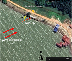
Figure 3. Sampling point at Pantai Punggur
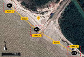
Figure 4. Sampling point at Pantai Perpat
2.2 Wave angle
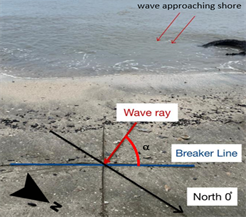
The wave angle at the breaker point refers to the angle at which ocean waves approach the shoreline as they begin to break in the nearshore zone [16]. This angle is critical because it influences how wave energy is distributed along the coast, particularly in driving longshore currents that transport sediment parallel to the shoreline [17]. The angle is measured between the wave crest direction and a line perpendicular to the coastline. When waves approach the shore obliquely, the resulting wave-induced current facilitates longshore sediment transport (LST), a major factor in shaping coastal morphology. In this study, the wave angle was determined using a protractor and a compass. The protractor was used to measure the wave angle, while the compass was essential for establishing the north–south axis. On-site, a line was drawn to represent the orientation of the shoreline, followed by another line indicating the direction of incoming waves, as illustrated in Figure 5. The wave angle is defined as the angle formed between these two lines. This angle is also commonly referred to as the deep water angle of incidence, denoted by α or θ, and becomes particularly important at the breaking point, where oblique wave approach drives longshore sediment transport.
Figure 5. Illustration of the determination of the wave angle
2.3 Sediment sampling
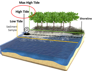
The first stage in soil testing involves the collection of soil samples, which form the foundation for laboratory analyses and test interpretation. The soil sampling for each coastal area was conducted, which consisted of eight (8) total samples, as shown in Figure 6. Disturbed soil samples were extracted using a hand auger for convenience and efficiency. In contrast, the collection of undisturbed samples required a sediment core extraction technique. Sampling procedures followed the guidelines established by the British Standard BS5930. Soil was extracted from depths ranging between 0.2 and 0.5 meters below the surface. At each designated sampling point, two replicate samples were collected to ensure representativeness and reduce potential variability. For laboratory testing, each sample was analyzed three times, and the average values were used in subsequent calculations to minimize random error and improve reliability. Each sample was immediately sealed in a labeled plastic bag and wrapped in several layers of cling film to preserve its natural moisture content. To retain the structural integrity of the samples, a polyvinyl chloride (PVC) tube served as the core container, maintaining a cylindrical shape. The PVC tube used had an inner diameter of 75 mm and a height of 200 mm. According to a study [12], tubes with diameters ranging from approximately 5 cm to 12 cm are typically employed in practice. The bulk density was determined by dividing the weight of the soil sample by its volume. It is essential to use undisturbed soil samples for the bulk density test to ensure accurate results, as maintaining their original form is crucial.
Figure 6. Illustration of the location of the sediment sample
2.4 Laboratory work
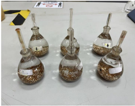
The laboratory analysis conducted in this study involved the physical testing of sediment samples that were collected from Pantai Parit Hailam, Pantai Punggur, and Pantai Perpat. The collected sediments were systematically sampled and examined to determine key physical properties, particularly porosity and bulk density. Specific gravity (Gs), a critical parameter in soil analysis, refers to the ratio of the density of soil particles to that of water, providing insights into the weight-volume relationship of the material [18]. The measurement of dry soil particle volume was carried out using a glass bottle filled with distilled water, into which the soil particles were gradually introduced. Following BS1377:1990:8.3, this test was designed to establish the average specific gravity (Gs), a fundamental metric for evaluating soil composition. To enhance accuracy and eliminate air bubbles within the soil matrix, this study employed the pycnometer method, with Figure 7 illustrating the apparatus utilized in the procedure.
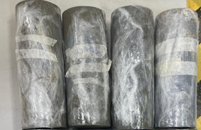
Bulk density, a widely recognized indicator of soil compaction, is determined by the ratio of the dry weight of the soil to its volume [19]. Several factors influence bulk density, including soil texture, mineral composition, organic matter content, and the structural arrangement of particles. For cohesive soil samples, the liner measurement method, as outlined in BS 1377: Part 2: 1990, was implemented to ensure precise assessment. This approach involves the collection of cylindrical samples to maintain their undisturbed state, as depicted in Figure 8. In this study, bulk density tests were systematically performed on samples retrieved from designated locations. Accurate measurements of each cylinder's weight, diameter, and height were recorded to calculate the volume. Since bulk density analysis requires maintaining the integrity of the soil structure, it is imperative to utilize undisturbed samples to achieve reliable results.
Figure 7. Soil sample and distilled water in pycnometers
Figure 8. Cylindrical soil samples were prepared for the bulk density test
Porosity (ρ), defined as the ratio of void volume to total soil volume, serves as an important parameter in assessing sediment packing and permeability characteristics [20]. In this study, porosity was not measured directly, but calculated from the relationship between bulk density (ρb) and particle density (ρs), following the procedures outlined in ASTM D7263 [21]. The particle density was obtained from the specific gravity test, while the bulk density was determined from oven-dried samples. The porosity value was then derived using the equation ρ = 1−(ρb/ρs). This indirect method has been widely applied in soil and sediment studies as it provides reliable estimates of porosity for coastal materials [22].
2.5 Data extraction-ECMWF
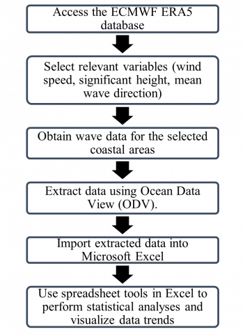
This study implemented data collection for capturing temporal variations in coastal hydrodynamics. ECMWF Reanalysis v5 (ERA5) is the fifth generation of atmospheric reanalysis produced by the European Centre for Medium-Range Weather Forecasts (ECMWF). The extraction of data from the ECMWF ERA5 dataset involved a systematic approach to ensure the accuracy and relevance of the data for this study. A total of 1224 data points were extracted for each sample location, corresponding to three-hourly records from May to September 2023. These data represent wave characteristics at the same locations listed in Table 1, focusing on three key variables: speed (meters/sec), significant wave height (meters), and mean wave direction (degrees). The dataset was limited spatially to three coastal areas (Pantai Parit Hailam, Pantai Punggur, and Pantai Perpat) with specific latitude and longitude ranges for each location and temporally to hourly records within the study period. Data were downloaded in NetCDF format, with manual extraction through the CDS web interface by selecting the required variables, region, and time.
Figure 9. Flowchart of the procedure to extract data from ECMWF
After extraction, the data underwent preprocessing to prepare it for analysis. The NetCDF files were imported into Ocean Data View (ODV) for visualization and quality control. During this step, missing values and anomalies were identified and corrected to ensure the reliability of the dataset. The processed data were then exported to Microsoft Excel for further analysis. Averages and trends of wave characteristics were computed to summarize the dataset and support visualization of spatial and temporal variability. The data used in this study were derived from raw data that were systematically organized from highest to lowest based on significant wave height values. The top one-third of the dataset, representing the highest waves, was selected, and the average of this subset was calculated to obtain the final representative values. This average corresponds to the significant wave height (Hs), a standard measure of the most energetic wave events in a record. This method ensures that the most impactful wave events are emphasized, providing a meaningful and accurate representation of wave dynamics for the study. Figure 9 shows a flowchart of a procedure to extract data from ECMWF.
2.6 Longshore sediment transport calculation
Calculating sediment transport necessitates specialized models and data collection methods tailored to the specific conditions of each coastal area. The CERC formula, which has been calibrated with field data from sandy beaches, is one of the most well-known methods for calculating the potential longshore sediment transport (LST) rate. Based on laboratory tests and field data, this formula created an empirical model considering significant wave height and wave angle, as detailed in Eq. (1). The key parameters used and source of data in the CERC equation are summarized in Table 2. Significant wave height (Hs) can be derived from data extracted from ECMWF. Hs measures the average height of the top one-third of waves in a given maritime environment. The data were analyzed using Microsoft Excel to determine significant values. Since the CERC model requires the breaking wave height (Hb) rather than deep-water Hs, a transformation process was applied. In the absence of detailed bathymetric data, the breaking depth (db) was estimated using the empirical relationship db = Hb/γ, where γ represents the breaker index. An iterative process was applied to transform Hs from deep water into Hb, a procedure commonly adopted in empirical wave transformation studies [8, 23, 24]. The empirical coefficient γ was assumed to be 0.78, following the widely accepted range of 0.70–0.80 for depth-limited breaking conditions [24, 25]. This assumption has been frequently applied in coastal engineering studies where site-specific bathymetry is not available, as it provides a reliable approximation of the depth at which wave breaking occurs [23, 26].
Furthermore, the data for sediment bulk density and sediment porosity can be gained from physical testing at the laboratory. The wave angle at the breaker was measured directly in the field. The LST was calculated in Microsoft Excel with the parameters for each sample point. According to the CERC approach, the longshore transport rate is expressed as follows:
$Q_V=k \frac{\rho_a \sqrt{g} / \gamma_b}{16\left(\rho_s-\rho_a\right)(1-p)} H_{s, b}^{5 / 2} \sin \left(2 \alpha_b\right)$ (1)
Table 2. CERC parameter
|
Parameter |
Definition |
Source of Data |
|
K |
Empirical coefficient (0.39) |
CERC standard value |
|
ρa |
Density seawater (1025 kg/m³) |
Standard ocean water density |
|
g |
Gravitational acceleration (9.81 m/s²) |
Constant |
|
$\gamma_b$ |
Wave breaking index (0.78) |
Literature (empirical value) |
|
ρs |
Sediment particle’s bulk density |
Laboratory test (sediment samples) |
|
p |
Porosity of the sediment particles |
Laboratory test (sediment samples) |
|
Hsb |
Sign. wave height at breaker point |
Transformed from ECMWF |
|
$ |
Angle of waves at breaker point |
Field measurement of shoreline orientation |
3.1 Wave angle
Wave angle refers to the direction at which waves approach the shoreline, playing a crucial role in influencing sediment transport and coastal dynamics [14]. This section presents the analysis of wave angle data, emphasizing its variations and potential impact within the study area. Table 3 summarizes the collected data, which includes the observation date, tide levels, and wave angles recorded at various sampling locations. Across all sampling points, the high tide level was consistently measured at 2.2 meters, while the low tide level was 0.5 meters, indicating a substantial tidal range during the study period. The wave angles, measured in relation to the shoreline, exhibited considerable variation, ranging from 15° to 60° depending on the sampling site. At Pantai Parit Hailam, wave angles were observed within the 45° to 60° range, whereas Pantai Punggur recorded lower values between 15° and 30°.
Table 3. Wave angle results
|
Sample Point |
Date |
High T. Level (m) |
Low T. Level (m) |
Wave Angle (°) |
Wave Approach (°) |
|
PH 1 |
5/06/23 |
10.56 am (2.2 m) |
5.02 pm (0.5 m) |
45 |
70 |
|
PH 2 |
5/06/23 |
10.56 am (2.2 m) |
5.02 pm (0.5 m) |
60 |
70 |
|
PG 1 |
6/06/23 |
11.38 am (2.2 m) |
5.43 pm (0.5 m) |
30 |
80 |
|
PG 2 |
6/06/23 |
11.38 am (2.2 m) |
5.43 pm (0.5 m) |
15 |
55 |
|
PG 3 |
6/06/23 |
11.38 am (2.2 m) |
5.43 pm (0.5 m) |
15 |
60 |
|
PP 1 |
1/06/23 |
8.15 am (2.2m) |
2.23 pm (0.7 m) |
25 |
40 |
|
PP 2 |
1/06/23 |
8.15 am (2.2m) |
2.23 pm (0.7 m) |
60 |
90 |
|
PP 3 |
5/06/23 |
10.56 am (2.2 m) |
5.02 pm (0.5 m) |
60 |
90 |
These differences underscore the spatial variability in wave approach, which is primarily influenced by local coastal topography and shoreline orientation. The spatial variability in wave angles at Pantai Parit Hailam and Pantai Punggur can be attributed to differences in coastal morphology and environmental conditions. Studies indicate that Pantai Punggur is characterized by a mild-sloped mudflat, which affects wave behavior and sediment transport [15]. Additionally, research on shoreline changes at Pantai Punggur highlights ongoing coastal erosion, which may further influence wave approach and angles.
3.2 Sediment properties
The analysis of sediment properties plays a crucial role in longshore sediment transport rate (LSTR) studies, as it helps develop effective management while providing a deeper understanding of sediment dynamics. In this study, a total of eight (8) soil samples were collected and analyzed, which focused on determining sediment characteristics at the sampling points. The results of this analysis are presented in tabular form to enhance clarity and comprehension, as shown in Table 4. The determination of specific gravity (G s) serves to establish its average value, which is crucial for analyzing the weight-volume relationship of sediments. In this study, the specific gravity was found to range between 2.78 and 2.96, reflecting the sediment composition in the examined coastal regions. These values closely align with the specific gravity of 2.6 reported by study [27], particularly in eroded coastal areas such as Pantai Punggur. This correlation reinforces the consistency of sediment composition across various coastal environments. Moreover, the sediment characteristics in Batu Pahat were influenced by moisture content variations between 70.1% and 122.6%, affecting both density and porosity [28]. These factors collectively contribute to the observed weight-volume relationships in coastal sediments.
Table 4. Sediment properties results
|
Sampling Point |
Specific Gravity |
Bulk Density (g/cm3) |
Porosity |
|
PH 1 |
2.79 |
1.16 |
0.55 |
|
PH 2 |
2.87 |
1.14 |
0.57 |
|
PG 1 |
2.78 |
1.14 |
0.55 |
|
PG 2 |
2.81 |
1.33 |
0.53 |
|
PG 3 |
2.96 |
1.28 |
0.57 |
|
PP 1 |
2.89 |
1.29 |
0.55 |
|
PP 2 |
2.80 |
1.30 |
0.54 |
|
PP 3 |
2.90 |
1.36 |
0.53 |
Soil bulk density is a fundamental property influenced by various physical and chemical factors, which continuously evolve with changes in soil structure. Among these factors, clay content plays a significant role in determining bulk density, second only to sand content. While silt concentration exhibits a negative correlation with bulk density, its impact is relatively indirect and less pronounced [29, 30]. The results presented in Table 4 indicate that the highest bulk density recorded is 1.36 g/cm³ at PP 3, whereas the lowest values of 1.14 g/cm³ were observed at PH 2 and PG 1. This variation is closely linked to the soil composition within the study area, where a higher proportion of clay and silt corresponds to lower bulk density. In contrast, sandy soils tend to exhibit higher bulk density due to their lower content of loose, permeable materials and organic matter, such as silt and clay [31]. Research suggests that sandy soils typically have bulk densities ranging from 1.4 to 1.7 g/cm³, whereas clay-rich soils tend to fall within the 1.0 to 1.3 g/cm³ range [32]. These findings reinforce the observed trends in bulk density variations across different soil types.
3.3 Coastal parameter
The European Centre for Medium-Range Weather Forecasts (ECMWF) produces numerical weather forecasts, monitors the Earth's system, conducts scientific and technical research to enhance forecasting accuracy, and maintains a comprehensive archive of meteorological data. Wind and wave data were retrieved from the ECMWF database at three-hour intervals, including measurements of wind speed, significant wave height, and mean wave direction as shown in Table 5. The recorded wind speeds across the sampling points range from 1.95 m/s to 1.99 m/s, indicating relatively consistent coastal wind conditions. The slight variations in wind speed may be attributed to localized factors such as topography, surface roughness, and proximity to coastal features. A study on coastal wind speed variability suggests that wind speeds near shorelines are influenced by seasonal trends, atmospheric pressure systems, and land-sea temperature differences [33]. The findings in the dataset align with observations from machine learning-based coastal wind predictions, which highlight that wind speeds in coastal environments exhibit minor fluctuations due to seasonal and diurnal variations [34]. These variations can impact wave height, sediment transport, and coastal erosion, making wind speed an essential parameter in coastal process studies.
Table 5. Coastal process parameter results
|
Sampling Point |
Coastal Process Parameter |
|||
|
Wind Speed (m/s) |
Significant Wave Height at Breaker Point (m) |
Mean Wave Direction |
||
|
Bearing (°) |
Directional Point |
|||
|
PH 1 |
1.95 |
0.31 |
226.51 |
SW |
|
PH 2 |
1.97 |
0.31 |
254.31 |
WSW |
|
PG 1 |
1.97 |
0.31 |
158.07 |
SSE |
|
PG 2 |
1.98 |
0.32 |
225.58 |
SW |
|
PG 3 |
1.98 |
0.32 |
226.15 |
SW |
|
PP 1 |
1.99 |
0.32 |
172.00 |
S |
|
PP 2 |
1.99 |
0.32 |
170.00 |
S |
|
PP 3 |
1.99 |
0.32 |
226.19 |
SW |
The recorded significant wave height (SWH) values, ranging between 0.31 m and 0.32 m, indicate relatively stable wave conditions across the study area. Significant wave height, which represents the average height of the highest one-third of waves in a given period, is a fundamental parameter in calculating LSTR. The observed values suggest a low-energy wave environment, which is typical for sheltered coastal areas or regions with limited wave fetch. Study [35] has shown that wave heights below 0.5 m are often associated with low sediment transport rates, reducing the impact of wave-induced erosion along the shoreline. Research on coastal storm dynamics suggests that regions experiencing significant wave heights below 0.5 m are generally less susceptible to extreme storm impacts, making them suitable for shoreline stabilization strategies and sediment retention initiatives. The findings from this study align with past observations from remote sensing and buoy-based wave monitoring [36], confirming that coastal wind speeds and seabed conditions play a major role in regulating wave behavior in nearshore environments.
The mean wave direction data extracted from ECMWF provides valuable insights into the dominant wave approach patterns along the coastlines of Pantai Parit Hailam, Pantai Punggur, and Pantai Perpat. The recorded wave bearings, ranging from 158.07° (SSE) to 254.31° (WSW), indicate a strong influence of the Southwest Monsoon (SWM), which predominantly drives waves from southwestern and southern quadrants during the peak monsoonal months. Additionally, waves bearing 170° to 172° (S) highlight localized influences such as tidal currents and coastal obstructions that contribute to wave refraction and directional variability [37]. These findings align with global ECMWF-based studies that demonstrate monsoonal wave patterns and their impacts on sediment dynamics. Coastal processes such as wave energy dissipation, sediment resuspension, and longshore transport are directly influenced by the prevailing wave direction, which determines shoreline stability and erosion rates. Previous studies on wave refraction and sediment transport modeling suggest that wave orientations in the 220° to 260° range are common in regions impacted by monsoonal weather systems, reinforcing the observed directional trends in the present dataset [38].
3.4 LSTR result
Estimating sediment transport in coastal regions requires the use of specialized models and data collection techniques that are adapted to site-specific coastal conditions. Among the most commonly applied methods for calculating longshore sediment transport rates (LSTR) is the Coastal Engineering Research Center (CERC) formula, as outlined in the Shore Protection Manual (1984). In this study, LSTR values were calculated using Eq. (1), assuming a constant empirical coefficient of 0.39 and a wave-breaking index of 0.78. These values were adopted based on previous laboratory and field studies, where 0.39 has been widely applied as the empirical coefficient in the CERC formula [8, 9], while 0.78 is generally used as the wave-breaking index under regular wave conditions [39]. The application of these constants is considered reasonable for the Batu Pahat coastline, which is characterized by sandy beaches and moderate wave energy conditions. According to data from the ECMWF, a wave approach direction of 0° indicates waves arriving from the north, while 90° corresponds to waves approaching from the east. The mean wave direction is critical in determining the direction of sediment transport along the coast, indicating whether movement occurs to the right or left of the shoreline [40].
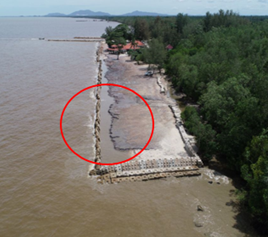
The observed LSTR values in the study area ranged from 0.0033 m³/s to 0.0062 m³/s, reflecting spatial variations in sediment movement along the coastline as shown in Table 6. LSTR is a critical indicator in coastal dynamics, representing the movement of sediments parallel to the shoreline due to the combined influences of wave energy, nearshore currents, and sediment characteristics. Higher LSTR values, such as 0.0062 m³/s recorded at station PH 1, suggest more intense sediment transport, likely driven by stronger wave forces or oblique wave approaches. In contrast, lower values, such as 0.0033 m³/s observed at PG 2, indicate reduced hydrodynamic activity or localized sediment retention. A possible explanation for the lower transport rate at PG 2 is the presence of a revetment structure (Figure 10), which acts as a physical barrier that dissipates wave energy. This effectively minimizes sediment displacement in the area, resulting in decreased LSTR values. Similar patterns have been identified in other studies, where coastal structures significantly influence local sediment dynamics [41].
The calculated LSTR values in this study (0.0033–0.0062 m³/s) fall within the low-to-moderate range compared with other coastal environments worldwide. Along the west coast of India, for instance, transport rates of 0.002–0.012 m³/s have been reported, reflecting variability linked to wave approach and nearshore morphology [42]. In contrast, higher-energy settings such as the Nile Delta, Egypt, often experience rates exceeding 0.01 m³/s due to stronger wave forcing [43]. These comparisons indicate that the Batu Pahat coastline exhibits transport dynamics typical of low-to-moderate energy coasts, where both natural conditions and coastal structures reduce sediment mobility.
Figure 10. Location of the revetment structure at PG 2 near the study area
Table 6. Longshore sediment transport rates results
|
Sampling Point |
LSTR (m³/s) |
|
PH 1 |
0.0062 |
|
PH 2 |
0.0044 |
|
PG 1 |
0.0061 |
|
PG 2 |
0.0033 |
|
PG 3 |
0.0034 |
|
PP 1 |
0.0053 |
|
PP 2 |
0.0061 |
|
PP 3 |
0.0058 |
Beyond energy levels, LSTR variability is also shaped by hydrodynamic and morphological factors such as wave direction, current velocity, and beach slope. In Malaysia, studies have shown that areas with reduced transport rates are more prone to sediment accumulation and altered shoreline morphology, necessitating stabilization measures like groynes and breakwaters [44]. Field data from other monsoonal coasts, such as India, further support this pattern, with reported LSTR values of 0.0025–0.0075 m³/s [45], closely matching the range found in Batu Pahat. This consistency reinforces the interpretation that sediment transport processes in the study area are governed by moderate wave forcing and localized engineering interventions, highlighting the need for carefully tailored coastal management strategies.
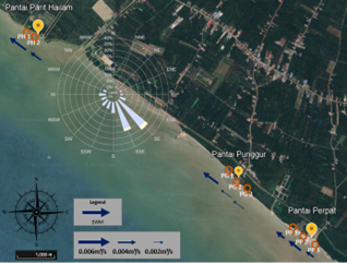
Figure 11 illustrates the longshore sediment transport rate (LSTR) across three coastal zones in Batu Pahat, accompanied by a wave rose diagram that displays significant wave height (SWH) and wave direction variations. The LSTR is represented by directional vectors, with the largest vector indicating the highest sediment transport rate, showing movement predominantly toward the left along the coastline. These vectors correspond with wave approaches from the southwest (SW), west-southwest (WSW), south-southeast (SSE), and south (S), demonstrating the influence of wave direction on sediment dynamics. The wave rose diagram further reveals dominant wave approach patterns from the southeast (SE) and south-southeast (SSE), with color-coded spokes indicating the frequency and magnitude of SWH. Wave activity not only governs sea surface hydrodynamics but also plays a significant role in shaping sediment transport and coastal morphology, while coastal geomorphology itself modulates the extent and direction of sediment movement along the shoreline. Previous studies on wave propagation models further support that these coastal wave patterns are strongly influenced by both bathymetric conditions and atmospheric forcing, reinforcing the observed directional consistency in wave approach from the SE and SSE sectors [46].
Figure 11. Illustration of dominant wave and wind directions driving longshore sediment transport
The dominance of waves approaching from the south and southeast sectors drives oblique wave incidence along the Batu Pahat shoreline, generating longshore currents that result in a net northward sediment transport. Prevailing winds from the south and southeast during much of the year produce wave trains that strike the coast at an oblique angle. This incidence angle introduces a strong alongshore component of wave energy, which subsequently induces northward-directed currents and promotes sediment movement parallel to the shoreline. Consequently, the overall sediment transport regime is biased northward, reflecting the direct influence of regional wind–wave forcing from the southern quadrants [47, 48].
This study demonstrated that longshore sediment transport along the Batu Pahat coast is predominantly northward, with calculated longshore sediment transport rates (LSTR) ranging between 0.0033 and 0.0062 m³/s. This represents the first quantitative assessment of LSTR in Batu Pahat using the CERC formula, providing a baseline reference for future coastal management in the region. Variations across the three study sites were linked to differences in coastal morphology, sediment properties, and the presence of revetments, with the highest transport rate observed at PH 1, indicating the highly dynamic nature of this sector. While a constant empirical coefficient of 0.39 and a wave-breaking index of 0.78 were applied following established literature, their uniform use across sites underscores the need for site-specific calibration in future applications of the CERC formula. Seasonal variability in sediment transport could not be conclusively validated in this study due to the single seasonal dataset; therefore, multi-seasonal monitoring is recommended to establish stronger evidence of monsoonal influence on LSTR.
Based on these findings, several practical recommendations are proposed. Given the strong northward transport and the highest LSTR at PH 1, a jetty or groyne system in this sector would likely be most effective in interrupting sediment drift and reducing erosion risk. Establishing a long-term monitoring program that integrates field measurements, remote sensing, and numerical modeling is also essential for tracking sediment dynamics and evaluating the effectiveness of erosion control measures.
This research was funded by Universiti Tun Hussein Onn Malaysia through Multidisciplinary Research Grant (MDR) (Vot Q695) and GPPS (Vot J183).
[1] Davidson-Arnott, R., Bauer, B., Houser, C. (2010). Introduction to Coastal Processes and Geomorphology. Cambridge: Cambridge University Press. https://doi.org/10.1017/9781108546126
[2] Zhang, K., Xuan, W., Bai, Y., Xu, X. (2021). Prediction of sediment transport capacity based on slope gradients and vegetation cover. PLoS ONE, 16(9): e0256827. https://doi.org/10.1371/journal.pone.0256827
[3] Chen, B., Zhang, X. (2022). Effects of slope vegetation patterns on erosion sediment yield and hydraulic parameters in slope-gully system. Ecological Indicators, 145: 109723. https://doi.org/10.1016/j.ecolind.2022.109723
[4] Masselink, G., Hughes, M., Knight, J. (2011). Introduction to Coastal Processes and Geomorphology (3rd ed.). Routledge. https://doi.org/10.4324/9780203785461
[5] Bosboom, J., Stive, M.J.F. (2021). Coastal Dynamics. TU Delft OPEN Books. https://doi.org/10.5074/T.2021.001
[6] Berman, G. (2011). Longshore Sediment Transport, Cape Cod, Massachusetts. Woods Hole Oceanographic Institution.
[7] U.S. Army Corps of Engineers. (1984). Shore Protection Manual. Coastal Engineering Research Center. https://usace.contentdm.oclc.org/digital/collection/p16021coll11/id/1934/.
[8] Komar, P.D., Gaughan, M.K. (1972). Airy wave theory and breaker height prediction. Coastal Engineering Proceedings, 1(13): 405-418. https://doi.org/10.1061/9780872620490.023
[9] Smith, E.R., Wang, P., Ebersole, B.A., Zhang, J. (2009). Dependence of total longshore sediment transport rates on incident wave parameters and breaker type. Journal of Coastal Research, 25(3): 675-683. https://doi.org/10.2112/07-0919.1
[10] Hayazi, F., Mat Zain, N.A., Mokhtar, M., Daud, M.E., Hamid, N.B., Bidoloh, S. (2025). Temporal correlation of shoreline changes and sediment properties along Batu Pahat, Johor Coastline. Journal of Advanced Research in Applied Mechanics, 138(1): 17-26.
[11] Department of Irrigation and Drainage. (2015). Coastal Management - Activities. https://www.water.gov.my/index.php/pages/view/515?mid=290.
[12] Department of Irrigation and Drainage. (2019). DID Basic Data and Information Compendium. https://www.water.gov.my/jps/modules_resources/bookshelf/kompendium_2019/kompendium_2019.pdf.
[13] Maulud, K.N.A., Rafar R.M. (2015). Determination the impact of sea level rise to shoreline changes using GIS. In 2015 International Conference on Space Science and Communication. pp 352-357. https://www.proceedings.com/content/027/027888webtoc.pdf.
[14] Siddiq, M.I., Daud, M.E., Kaamin, M., Mokhtar, M., Omar, A.S., Duong, N.A. (2022). Investigation of Pantai Punggur coastal erosion by using UAV photogrammetry. International Journal of Nanoelectronics and Materials, 15: 61-69. https://www.researchgate.net/publication/359864547.
[15] Mokhtar, M. (2023). A new formulation for assessing coastal erosion and morphology change in the sand-mud beach area. Ph.D. thesis, Universiti Tun Hussein Onn Malaysia.
[16] Agbetossou, K.S.F., Aheto, D.W., Angnuureng, D.B., van Rijn, L.C., Houédakor, K.Z., Brempong, E.K., Tomety, F.S. (2023). Field measurements of longshore sediment transport along Denu Beach, Volta Region, Ghana. Journal of Marine Science and Engineering, 11(8): 1576. https://doi.org/10.3390/jmse11081576
[17] Lim, C.B., Lee, J.L. (2018). Performance test of parabolic type equilibrium shoreline formula using wave data observed in East Sea. Journal of Ocean Engineering and Technology, 32(2): 123-130. https://doi.org/10.26748/KSOE.2018.4.32.2.123
[18] Ciccaglione, M.C., Buccino, M., Calabrese, M. (2023). On the evolution of beaches of finite length. Continental Shelf Research, 259: 104990. https://doi.org/10.1016/j.csr.2023.104990
[19] Li, S., Chen, X., Zhou, G., Song, D., Chen, J. (2018). Influence of bulk density and slope on debris flows deposit morphology: Physical modelling. In Proceedings of China-Europe Conference on Geotechnical Engineering, pp. 1495-1499. https://doi.org/10.1007/978-3-319-97115-5_131
[20] Das, B.M. (2014). Principles of Geotechnical Engineering. Cengage Learning. Cengage. https://www.cengage.ca/c/etextbook-principles-of-geotechnical-engineering-10e-das/9780357711606/.
[21] ASTM. (2021). Standard Test Methods for Laboratory Determination of Density (Unit Weight) of Soil Specimens. Standard D7263-21. ASTM International.
[22] Budhu, M. (2011). Soil Mechanics and Foundations (3rd ed.). Wiley and Sons.
[23] Kamphuis, J.W. (2010). Introduction to Coastal Engineering and Management (2nd ed.). World Scientific.
[24] Lee, K.H., Cho, Y.H. (2021). Simple breaker index formula using linear model. Journal of Marine Science and Engineering, 9(7): 731. https://doi.org/10.3390/jmse9070731
[25] Zhang, C., Li, Y., Cai, Y., Shi, J., Zheng, J., Cai, F., Qi, H. (2021). Parameterization of nearshore wave breaker index. Coastal Engineering, 168: 103914. https://doi.org/10.1016/j.coastaleng.2021.103914
[26] U.S. Army Corps of Engineers. (2002). Coastal engineering manual (EM 1110-2-1100). Washington, D.C.: U.S. Army Corps of Engineers. https://plainwater.co/pubs/EM1110-2-1100P1.pdf.
[27] Mokhtar, M., Ariffin, M.A.F.B., Daud, M.E., Kaamin, M., Azmi, M.A.M., Hamid, N.B. (2022). Sediment properties of eroded coastal area at Batu Pahat, Johor, Malaysia. Environment and Ecology Research, 10(2): 248-225. https://doi.org/10.13189/eer.2022.100214
[28] Mokhtar, M., Daud, M.E., Kaamin, M., Noor, H., et al. (2023). Beach profile and shoreline sediment properties at eroded area in Batu Pahat. Construction Technologies and Architecture, 4: 127-137. https://doi.org/10.4028/p-ny3700
[29] Askin, T., Özdemir, N. (2003). Soil bulk density as related to soil particle size distribution and organic matter content. Poljoprivreda, 9: 52-55.
[30] Cicek, B. (2022). Revisiting vernacular technique: Engineering a low environmental impact earth stabilisation method. Ph.D. thesis. Bauhaus-Universität Weimar. https://doi.org/10.25643/bauhaus-universitaet.4698
[31] Guruprasad, M.H., Soraganvi, V.S. (2014). Impact of soil organic carbon on bulk density and plasticity index of arid soils of Raichur, India. International Research Journal of Environment Sciences, 3(2): 48-58.
[32] Singh, P.D., Kumar, A., Dhyani, B.P., Kumar, S., Shahi, U.P., Singh, A., Singh, A. (2020). Relationship between compaction levels (bulk density) and chemical properties of different textured soil. International Journal of Chemical Studies, 8(5): 179-183. https://doi.org/10.22271/chemi.2020.v8.i5c.10294
[33] Wang, L., Fu, A., Bashir, B., Gu, J., Sheng, H., Deng, L., Deng, W., Alsafadi, K. (2024). Characteristics and driving mechanisms of coastal wind speed during the typhoon season: A case study of Typhoon Lekima. Atmosphere, 15(8): 880. https://doi.org/10.3390/atmos15080880
[34] Durap, A. (2025). Interpretable machine learning for coastal wind prediction: Integrating SHAP analysis and seasonal trends. Journal of Coastal Conservation, 29: 24. https://doi.org/10.1007/s11852-025-01108-y
[35] Afzal, M.S., Kumar, L., Chugh, V., Kumar, Y., Zuhair, M. (2023). Prediction of significant wave height using machine learning and its application to extreme wave analysis. Journal of Earth System Science, 132: 51. https://doi.org/10.1007/s12040-023-02058-5
[36] Mitsopoulos, P., Peña, M. (2023). Characterizing coastal wind speed and significant wave height using satellite altimetry and buoy data. Remote Sensing, 15(4): 987. https://doi.org/10.3390/rs15040987
[37] Gujjar, A.R., Angusamy, N., Rajamanickam, G.V. (2008). Wave refraction patterns and their role in sediment redistribution along South Konkan, Maharashtra, India. GeoActa, 7: 69-79.
[38] Jayaraj, V.J., Chandrasekar, N., Jayangondaperumal, R., Thakur, V.C., Purniema, K.S. (2019). An interpretation of wave refraction and its influence on foreshore sediment distribution. Acta Oceanologica Sinica, 38: 151-160. https://doi.org/10.1007/s13131-019-1446
[39] Kamphuis, J.W. (1991). Alongshore sediment transport rate. Journal of Waterway, Port, Coastal, and Ocean Engineering, 117(6): 624-641. https://doi.org/10.1061/(ASCE)0733-950X(1991)117:6(624)
[40] Casas-Prat, M., Sierra, J.P. (2012). Trend analysis of wave direction and associated impacts on the Catalan coast. Climatic Change, 115(3): 667-691. https://doi.org/10.1007/s10584-012-0466-9
[41] Fitri, A., Hashim, R., Abolfathi, S., Abdul Maulud, K.N.A. (2019). Dynamics of sediment transport and erosion deposition patterns in the locality of a detached low crested breakwater on a cohesive coast. Water, 11(8): 1721. https://doi.org/10.3390/w11081721
[42] Chandramohan, P., Nayak, B.U. (1992). Longshore sediment transport model for the Indian west coast. Journal of Coastal Research, 8(4): 775-787. http://drs.nio.org/drs/handle/2264/3103
[43] Frihy, O.E., Deabes, E.A., El‑Sayed, W.R. (2003). Processes reshaping the Nile delta promontories of Egypt: pre‑ and post‑protection. Geomorphology, 53(3‑4): 263-279. https://doi.org/10.1016/S0169-555X(02)00318-5
[44] Fitri, A., Hashim, R., Abolfathi, S., Abdul Maulud, K.N. (2019). Dynamics of sediment transport and erosion deposition patterns in the locality of a detached low crested breakwater on a cohesive coast. Water, 11(8): 1721. https://doi.org/10.3390/w11081721
[45] Chandramohan, P., Jena, B.K., Kumar, V.S. (2001). Littoral drift sources and sinks along the Indian coast. Current Science, 81(3): 292-297.
[46] Clementi, E., Oddo, P., Drudi, M., Pinardi, N., Korres, G., Grandi, A. (2017). Coupling hydrodynamic and wave models: First step and sensitivity experiments in the Mediterranean Sea. Ocean Dynamics, 67(10): 1293-1312. ttps://doi.org/10.1007/s10236-017-1087-7
[47] Rashidi, A.H.M., Jamal, M.H., Hassan, M.Z., Sendek, S.S.M., Sopie, S.L.M., Abd Hamid, M.R. (2021). Coastal structures as beach erosion control and sea level rise adaptation in Malaysia: A review. Water, 13(13): 1741. https://doi.org/10.3390/w13131741
[48] Ramli, N.I., Ramesh, Y. (2018). Assessment of coastal erosion related to wind characteristics in Peninsular Malaysia. Journal of Engineering Science and Technology, 13(11): 3677-3690. http://jestec.taylors.edu.my/Vol%2013%20issue%2011%20November%202018/13_11_17.pdf.