Sara Boutouhami*![]() | Oualid Mecili
| Oualid Mecili![]() | Farid Nouioua
| Farid Nouioua![]()
© 2025 The authors. This article is published by IIETA and is licensed under the CC BY 4.0 license (http://creativecommons.org/licenses/by/4.0/).
OPEN ACCESS
Diabetic retinopathy (DR) is a common microvascular problem of diabetes. Early examination and treatment of this problem can efficiently moderate its risk. Therefore, a robust and automated diagnosis system is essential and very important in this context. The first advances in fully automated methods based on diagnostics have already revolutionized the way of detecting and identifying DR. However, further exciting advances are still possible. For example, using fuzzy rules, explainable methods, fully data driven models, and deep learning models. Based on the considered fundus images, we propose in this paper an explainable classification model based on the ALMMo-0 classifier that used the CLAHE technique as a preprocessing method and the VGG16 deep feature to improve the DR diagnosis in terms of robustness by using supervised fuzzy learning. The deep features obtained from VGG16 are used as the input vector for the ALMMo-0 classifier. The model is evaluated with several DR datasets and data augmentation techniques. The proposed ALMMo-0 classifier-based model for the detection of DR achieves high accuracy scores of 0.87 on MESSIDOR-2, 0.93 on APTOS-2019, and 0.97 on IDRiD, along with excellent sensitivity (0.88 on MESSIDOR-2, 0.92 on APTOS-2019, and 0.96 on IDRiD) and specificity (0.98 on MESSIDOR-2, 0.93 on APTOS-2019, and 0.98 on IDRiD) scores. Moreover, further comparative study demonstrates the effectiveness of the proposed model.
diabetic retinopathy classification, ALMMo-0 classifier, fuzzy rule-based system, explainable AI, deep learning
Diabetic retinopathy (DR) is a dangerous optical illness concerning diabetes and it is a well-known cause of blindness [1]. An early diagnosis of DR requires an effective screening procedure. Systematic screening for diabetes can decrease the danger of blindness. Nevertheless, DR diagnosis is an intensive process. Therefore, computer aided diagnosis models for DR are indispensable. Numerous diagnosis models of DR based on machine learning techniques (ML) have been planned for automatic diabetic retinopathy classification [2-5]. In these models, the fundamentals of a computer-aided diagnosis system have been employed. In ML techniques, the data is essential and crucial for training the classifiers [6]. Various fully automatic models of DR classification based on deep learning have been widely used and have reached state-of-the-art performance.
Frequent deep learning methods suffer from the absence of explanation and are strongly influenced by training parameters. The explanation and robustness need enhancement to make other classification approaches more explainable for diabetic retinopathy.
Fuzzy rule-based learning (FRBL) is an alternative approach to enhance the robustness and explainability of the classification task. However, it has not been yet applied for the diabetic retinopathy classification problem.
The motivation behind the use of fuzzy rule-based learning is that, rather than classical classifiers, it is based on interpretable and easy to understand if-then fuzzy rules to classify an object. Hence, FRBL is an excellent tool in the medical diagnosis context where it is crucial to be able to explain the decisions made by doctors. In addition, this kind of models naturally contracts with uncertainty and imprecision. Besides, FRBL generally achieves high classification accuracy which is a motivating point for doctors. So, in order to enhance the robustness, the effectiveness and the explainability of the proposed model, we apply in this paper the ALMMo-0 classifier, which is based on fuzzy learning, to classify the fundus images. The performance and robustness results of the proposed solution are computed and discussed.
The remainder of this paper is organized as follows: The related work is described in Section 2. This section also discusses the motivation of this work by identifying the research gaps to be addressed. Section 3 is devoted to the classification approach based on ALMMo-0 classifier and its modeling method. The description of the main steps involved in our proposed system is presented in Section 4. The experimental validation of the proposed model is described and discussed in Section 5. Finally, Section 6 concludes the paper and gives some directions for future work.
Diabetic retinopathy (DR) is a leading cause of preventable blindness among diabetic patients, necessitating early detection and treatment. Manual diagnosis requires significant time and resources, prompting the development of automated detection and classification methods using deep learning techniques [7]. These approaches analyze retinal fundus images to detect blood vessels, hemorrhages, and other DR-related features. Various machine learning algorithms and deep learning models, have been employed to classify DR stages with high accuracy.
The autonomous learning multi-model classifier of 0-order (ALMMo-0) is a noniterative, data-driven classifier that automatically extracts data clouds and forms, for each class, sub-classifiers based on fuzzy rules [8]. While originally parameter-free, a new approach introduces an initial radius hyper-parameter, allowing users to choose between accuracy and complexity [9]. The ALMMo-0 system has been extended to first-order (ALMMo-1) and adapted for multi-class classification tasks, demonstrating flexibility and comparable performance to benchmark methods [10]. Both ALMMo-0 and ALMMo-1 systems have shown high accuracy and efficiency in classification and regression tasks, with the ability to learn from streaming data and self-evolve their structure. These characteristics make ALMMo systems attractive solutions for various real-world applications, offering a balance between performance and adaptability.
The xDNN model achieves a high accuracy of 99.7% on the APTOS-2019 dataset, emphasizing the importance of interpretability in clinical applications [11].
One study reported a deep learning model achieving 94% sensitivity and 98% specificity in DR detection [10]. These automated systems show promise in reducing vision loss by enabling timely referrals to ophthalmologists for further evaluation and treatment [12].
Combining CNNs with techniques like Adaptive Gabor Filters and Random Forests has improved classification accuracy to nearly 98% [13]. Recent models utilize attention mechanisms and vision transformers to enhance feature extraction, achieving accuracies of 99.63% [14].
Transfer learning has been widely used for DR detection. The work presented in the study [15] proposes a model for DR detection based on transfer learning. Bodapati et al. [16] combine feature extraction and transfer learning techniques. Bhardwaj et al. [17] developed a deep learning model to distinguish DR disease identification and its grading using a transfer learning approach. Pour et al. [18] performed feature extraction and classification in DR detection by using EfficientNet.
Jena et al. [19] proposed a novel approach for DR screening using asymmetric deep learning features, achieving 98.6% accuracy on the APTOS dataset and 91.9% on the MESSIDOR dataset. Nur-A-Alam et al. [20] introduced an automated technique for classifying retinal fundus images into DR and normal states using feature fusion, achieving a detection accuracy of 95.75%. Incir and Bozkurt [21] used K-Means clustering for lesion segmentation and pretrained models like EfficientNetV2-M, achieving 95.16% accuracy.
Omer [22] presented a computer-aided screening system (DREAM) utilizing a bilayered neural network for classifying DR severity, achieving 98.5% accuracy on 6,332 fundus images. Akhtar et al. [23] proposed a binary classification framework for DR detection using Transfer Learning, achieving a test accuracy of 97.82% with an image dataset from APTOS-2019. In the reference [24], machine learning algorithms such as logistic regression, naive bayes (NB), support vector machine (SVM) and random forest are used for DR detection and classification.
Table 1. Summary of models and results obtained by related works
|
Reference |
Method / Model |
Dataset |
Performance |
|
Mecili et al. [11] |
xDNN model |
APTOS-2019 |
99.7% accuracy |
|
Gargeya and Leng [12] |
Deep learning model |
- |
94% sensitivity, 98% specificity |
|
Thanikachalam et al. [13] |
CNN + Adaptive Gabor Filters + Random Forests |
- |
98% accuracy |
|
Ainapur and Patil [14] |
Attention mechanisms + Vision Transformers |
- |
99.63% accuracy |
|
Le et al. [15] |
Transfer learning model |
- |
- |
|
Bodapati et al. [16] |
Transfer learning + Feature extraction |
- |
- |
|
Bhardwaj et al. [17] |
Transfer learning for DR grading |
- |
- |
|
Pour et al. [18] |
EfficientNet for feature extraction |
- |
- |
|
Jena et al. [19] |
Asymmetric deep learning features |
APTOS, MESSIDOR
|
98.6% (APTOS), 91.9% (MESSIDOR) |
|
Nur-A-Alam et al. [20] |
Feature fusion for classification |
- |
95.75% accuracy |
|
Incir and Bozkurt [21] |
K-Means + EfficientNetV2-M |
- |
95.16% accuracy |
|
Omer [22] |
Bilayered neural network (DREAM) |
6,332 fundus images |
98.5% accuracy |
|
Akhtar et al. [23] |
Transfer learning for binary classification |
APTOS-2019 |
97.82% accuracy |
|
Manasa et al. [24] |
SVM, logistic regression, random forest, NB |
- |
- |
|
Costaner et al. [25] |
LBP + Wavelet transform + SVM |
- |
95.59% accuracy, 96% precision, 97.96% recall |
Costaner et al. [25] developed a machine learning-based method for DR detection using local binary pattern (LBP) and wavelet transform, achieving 95.59% accuracy, 96% precision, and 97.96% recall with SVM classification. Table 1 summarizes the related works for the DR automatic detection tasks.
Recent research on Transformer-based architectures for diabetic retinopathy (DR) classification has demonstrated impressive results, particularly in improving feature representation and global contextual understanding. For instance, Li and Huang [26] proposed a vision transformer (ViT)-based model that achieved an accuracy of 93.8% and an AUC of 0.97 on the EyePACS dataset, showing strong robustness in detecting different DR severity levels. Similarly, Dosovitskiy [27] highlighted the superior generalization ability of Transformer backbones over CNNs like ResNet50 and VGG16, reporting state-of-the-art results in image recognition tasks with accuracies exceeding 90% in medical imaging benchmarks. In another study, Xu and Wang [28] employed a Swin Transformer-based hierarchical network that reached 95.2% accuracy and an F1-score of 0.94 on the APTOS 2019 dataset, particularly excelling in identifying subtle lesion regions and inter-class boundaries.
Current research on detecting and classifying diabetic retinopathy (DR) by using explainable methods reveals several critical gaps that hinder advancements in accurate diagnosis and treatment. While recent studies have made significant strides using deep learning, AI technologies, and explainable AI (XAI), the integration of these methods into practical clinical applications remains underexplored. There is a pressing need for comprehensive methodologies that effectively integrate various components to address these challenges. Key gaps include:
To address these gaps, future research should focus on developing comprehensive, intuitive, and clinically relevant frameworks that balance accuracy and explainability. This perspective highlights a potential trade-off between model performance and the clarity of explanations provided to clinicians, underscoring the need for a balanced approach in future research.
In the reference [8], the authors introduced the ALMMo-0 system within the empirical data analytics (EDA) framework [37]. EDA is a data-driven approach that focuses on extracting meaningful patterns and insights from empirical data without relying on strict assumptions about the underlying data distribution. It is particularly useful for handling complex, real-world datasets where traditional statistical methods may fall short.
The ALMMo-0 Classifier is an innovative approach to classification, developed as part of ongoing research in evolving and autonomous intelligent systems. This classifier, created by Professor Plamen Angelov and his team, is designed to operate in a dynamic and adaptive manner, addressing the limitations of traditional machine learning models that require extensive manual tuning and static structures. The ALMMo-0 classifier belongs to a family of models that emphasize autonomy, interpretability, and real-time adaptability, making it highly suitable for applications in environments where data evolves continuously.
Core Principles and Architecture. The ALMMo-0 classifier is built upon the foundations of the 0-Order AnYa Fuzzy Rules, which is known for its simplicity and direct data-driven approach. Unlike traditional machine learning models that often require iterative training processes and complex optimization, ALMMo-0 operates in a non-iterative, feedforward manner. This means that the model does not require repeated cycles of learning to improve performance; instead, it learns directly from the data as it arrives. The classifier is fundamentally data-driven, forming its structure based on the incoming data without the need for predefined parameters or extensive human intervention.
Data Clouds and Fuzzy Rules. A distinctive feature of the ALMMo-0 classifier is its ability to automatically extract data clouds from the dataset for each class. These data clouds represent clusters or groupings of data points that share similar characteristics. The classifier uses these clouds as the basis for generating fuzzy rules, which are central to its decision-making process. These fuzzy rules are of 0-order, meaning they are simple and do not involve complex mathematical functions, making them both efficient and interpretable. The use of data clouds allows the classifier to capture the inherent structure of the data in a way that is both flexible and robust.
Classification Strategy. When presented with new data, the ALMMo-0 classifier employs a "winner takes all" strategy to determine the class of the data point. This approach involves comparing the new data point against the established data clouds for each class. The classifier then generates confidence scores based on how well the new data fits into these clouds. The class with the highest confidence score is selected as the predicted class. This strategy not only ensures accurate classification but also provides a degree of confidence in each prediction, which can be crucial in applications where decision certainty is important.
Interpretability and Explainability. One of the key advantages of the ALMMo-0 model is its focus on explainability. In an era where artificial intelligence is increasingly being deployed in critical domains such as healthcare, finance, and autonomous systems, the ability to understand and trust the decisions made by AI systems is paramount. The ALMMo-0 classifier addresses this need by producing models that are inherently interpretable. The use of simple, 0-order fuzzy rules derived directly from data clouds allows users to understand the reasoning behind each classification decision. This transparency is vital in gaining the trust of end-users and ensuring that AI systems can be integrated seamlessly into decision-making processes.
Applications and Impact. The ALMMo-0 classifier is particularly well-suited for applications in dynamic environments where data is constantly evolving, and where models need to adapt in real-time. It is able to autonomously learn from data without requiring manual updates, which makes it ideal for scenarios such as real-time monitoring systems, adaptive control systems, and other applications where traditional static models may fail to keep pace with changing conditions. Additionally, the model’s explainability makes it valuable in fields where understanding the decision process is as important as the decision itself, such as in regulatory environments or areas requiring high levels of accountability.
In summary, the ALMMo-0 classifier represents a significant advancement in the field of autonomous and explainable AI. Its combination of non-iterative learning, real time adaptability, and interpretability sets it apart from more conventional machine learning approaches, making it a powerful tool for tackling complex, dynamic problems in numerous applications.
The general architecture of our proposal consists of several key components, as shown in Figure 1. These components work together to process empirical data, generate fuzzy rules, and optimize models using the EDA framework.

Figure 1. ALMMo-0 system: general architecture
4.1 Preprocessing
Pre-processing fundus images is a crucial step used to reduce noise and inconsistencies from different imaging devices and environments. Techniques like resizing, cropping, contrast adjustment, normalization, and data augmentation applied to enhance image quality. This guarantees classification models emphasis on key features, improving accuracy and robustness in term of classification performance. Particularly in diabetic retinopathy detection, it leads to more reliable and consistent medical image analysis.
Diabetic retinopathy datasets frequently contain fundus images with different resolutions and aspect ratios, sometimes containing black space. To normalize input sizes, cropping image is applied to eliminate useless areas. This ensures images with fixed resolution, which permit to enhancing classification model performance. In addition, CLAHE (Contrast Limited Adaptive Histogram Equalization) method [38] efficiently enhances image quality by improving low-contrast areas. It highlights lesions in fundus images (FIs), making medical image analysis more reliable.
Also, CLAHE enhances local contrast, making subtle details more visible in regions where there are significant variations of intensity levels. One main parameter of CLAHE method is the clip limit: It regulates the contrast adjustment process. Besides, the clip limit parameter plays an important role in balancing image clarity with preservation of details. This user-defined value modifies the histogram to prevent excessive distortion. As a result, good tuning guarantees effective improvement without over-amplifying noise or artifacts.
Data augmentation generates diverse training samples through transformations such as rotation, flipping, scaling, and brightness adjustment, thereby improving model robustness and generalizability.
Finally, normalization standardizes pixel values, scaling them to a consistent range (e.g., [0, 1] or zero mean and unit variance), which stabilizes training and ensures faster convergence.
Together, these preprocessing steps: Circle cropping, CLAHE, data augmentation and normalization, create a robust foundation for accurate and reliable DR detection and classification. Figure 2 shows some examples of original and preprocessed images.

Figure 2. Examples of some preprocessed and original fundus images, associated with their respective classes
4.2 Feature extraction
In computer vision, obtaining relevant features from traits plays a vital role in tasks like object detection, content-based retrieval, and image classification. Deep learning has revolutionized this process by offering advanced methods for feature extraction, particularly leveraging pre-trained CNNs, a widely used approach is transfer learning which enables the adaptation of knowledge from pre-trained models to new applications. Rather than constructing a deep neural network from the ground up, we can utilize a model trained on extensive datasets like ImageNet and fine-tune to enhance performance on specific tasks This approach is especially useful when working with smaller datasets or when computational resources are limited. Transfer learning has been successfully applied in various medical diagnostics, such as developing a cloud-based solution for liver cancer detection using deep learning and classifying cancer from DNA microarray data with genetic algorithms and case-based reasoning. These examples demonstrate how transfer learning can enhance the adaptability and effectiveness of models across different healthcare applications.
One well-known network frequently applied in transfer learning is VGG16, which achieved prominence during the ImageNet Large Scale Visual Recognition Challenge (ILSVRC) due to its impressive accuracy. Developed by the Visual Geometry Group at the University of Oxford, VGG16 is a deep convolutional neural network featuring 16 layers and utilizing small 3´3 convolutional filters consistently. It’s simple yet effective architecture, along with strong performance on ImageNet, has made it a widely adopted choice for numerous computer vision applications. The VGG16 architecture includes several convolutional layers followed by maxpooling layers, leading up to fully connected layers. After the final convolutional layer, which produces a 7´7´512 tensor, the output is flattened into a single-dimensional vector of length 25,088. This vector is then passed through fully connected layers, where it is reduced to a 1´4096-dimensional vector through matrix multiplication and a ReLU activation function.
In transfer learning, VGG16 functions as a feature extractor by retaining its convolutional layers and removing the fully connected layers. This adaptation allows the network to process images and generate a 1´4096-dimensional feature vector. The process involves image pre-processing, passing it through the modified network, and extracting meaningful features. This method enables efficient feature extraction without requiring extensive retraining. Typically, VGG16 uses weights pre-trained on the ImageNet dataset, which captures a broad range of visual features useful for various tasks. If the application domain differs significantly from ImageNet, additional domain-specific pretraining or fine-tuning may be required. However, in many cases, the default ImageNet weights suffice for feature extraction, unless the domain images are vastly different. In our experience, using the ImageNet weights yielded the best results, likely due to the diverse and rich feature representations learned from the extensive ImageNet dataset.
4.3 ALMMo-0 classifier
This section briefly recalls the main notions related to the 0-order AnYa Fuzzy Rule-Based (FRB) system and the EDA estimator. The AnYa FRB system is a type of fuzzy rule-based model that uses data clouds to represent rules, eliminating the need for predefined membership functions. This makes the system highly adaptive and capable of handling non-linear and dynamic data. The EDA estimator, on the other hand, is a computational tool used within the EDA framework to estimate parameters and optimize models based on empirical data. The AnYa Fuzzy rule-based system and the EDA estimator provide Together a flexible and efficient approach for modeling complex systems.
4.3.1 0-Order AnYa fuzzy rule-based system
The ALMMo-0 classification consists of a collection of AnYa fuzzy rules [8]. Unlike the commonly used Mamdani and Assilian [39], Zadeh [40] and Takagi and Sugeno [41] fuzzy rule-based (FRB) systems, in an AnYa fuzzy rule, the antecedent is simplified into a vector representing the focal points corresponding to the different data clouds. The concept of data clouds refers to clusters of data samples with shared characteristics, organized around focal points similar to Voronoi tessellation [42]. In the AnYa approach, the data clouds as well as their focal points serve as the foundation for the antecedent, i.e., the IF part, of the fuzzy rule. A zero-order AnYa fuzzy rule is formulated as follows:
Rule $i$ : IF $x \approx x_i^*$ $THEN \,Label$${ }_i$ (1)
where, $x_i^*$ is the focal point of the $i^{\text {th }}$ cloud; $L a b e l_i$ is the corresponding label. When classification is considered, inference in the 0-order AnYa rule of is done based on the principle "winner takes all".
4.3.2 EDA estimator
In the present paper, the EDA framework, and especially the unimodal density, is used as the main estimator to autonomously reveal global properties from observed data. We define the dataset or data stream in the Euclidean space $\mathbb{R}^d$ as $\left\{x_1, x_2, \ldots, x_k\right\}$, where subscripts denote time instances of data observation. For simplicity, Euclidean distance is used in the mathematical formulation, though other distance metrics can also be applied. The unimodal density of the ith data sample at the kth time instance is computed as:
$D_k\left(x_i\right)=\frac{1}{1+\frac{\left\|x_i-\mu_k\right\|^2}{\sigma_k^2}}=\frac{1}{1+\frac{\left\|x_i-\mu_k\right\|^2}{X_k-\left\|\mu_k\right\|^2}}$ (2)
where, $\mu_k$ is the mean of all the samples computed at the $k^{t h}$ time instance and $X_k$ is the average scalar product: $\sigma_k^2=X_k- \left\|\mu_k\right\|^2$. It is worth noting that in the case of Euclidean distance, the unimodal density has the form of a Cauchy function, even if there is no assumption that the distribution is a Cauchy distribution.
For efficient streaming data processing, recursive computation plays a fundamental role in optimizing memory usage and computational performance. The values of $\mu_k$ and $X_k$ are updated by using Eqs. (3) and (4), that recursively compute the unimodal density without explicit loops:
$\mu_k=\frac{k-1}{k} \mu_{k-1}+\frac{1}{k} x_k ; \quad \mu_1=x_1$ (3)
$X_k=\frac{k-1}{k} X_{k-1}+\frac{1}{k}\left\|x_k\right\|^2 ; \quad X_1=\left\|x_1\right\|^2$ (4)
4.3.3 Overview of multiple model architecture
This architecture utilizes multiple sub-classifiers to process incoming data samples within a classification framework. We evaluate every new data sample, $x_k$, by all available subclassifiers. Each sub-classifier $i$ produces a confidence score, $\lambda_i$, representing the probability that $x_k$ belongs to a particular class. The final classification is determined using a "winner-takes-all" approach, where $x_k$ is assigned to the class with the highest confidence score.
Label $=\operatorname{argmax}_{i=1,2, \ldots, R}\left(\lambda_i\right)$ (5)
This multiple-model approach enhances the classifier’s capacity for handling complex problems by combining the strengths of each sub-classifier as shown in Figure 3.

Figure 3. A conceptual framework diagram of a multiple-model classifier
4.3.4 Learning stage in the ALMMo-0 classifier
During the learning phase, we only update the AnYa fuzzy rule-based (FRB) rules relaying on new data sample’s class with normalizing these new samples:
$x_k \leftarrow \frac{x_k}{\left\|x_k\right\|}$ (6)
In the case of high-dimensional data, this normalization improves the classifier's performance. Let $x_k^i$ be a new data sample from class $i$. We update $\mu_{k-1}^i$, which denotes the class's global mean, to a new mean $\mu_k^i$. Since each data sample is normalized, the update of the average scalar product is not necessary.
The found focal points of class $i$, denoted as $x_j^{* i}$ for $j= 1,2, \ldots, F_i$ (where $F_i$ is the number of focal points) as well as the unimodal densities of the new data sample $x_k^i$ are computed using the following Eq. (7):
Dendity $=f\left(x_k^i, x_j^{*_i}\right)$ (7)
This density computation helps the classifier to effectively adapt itself to changing data distributions, particularly in high-dimensional spaces.
To determine if $x_k^i$ should create a new data cloud or a new rule, the following condition (Condition 1) is checked:
$\operatorname{IF}\binom{\left(D_k\left(x_k^i\right)>\max _{j=1,2, \ldots, F_i}\left(D_k\left(x_j^{* i}\right)\right)\right)}{\operatorname{OR}\left(D_k\left(x_k^i\right)>\max _{j=1,2, \ldots, F_i}\left(D_k\left(x_j^{* i}\right)\right)\right)}$ THEN Add $x_k^i$ as a novel focal point (8)
In the case where Condition 1 holds, a new fuzzy rule or data cloud is constructed and associated with $x_k^i$. The adaptation of the parameters of this new data cloud is done as follows:
$\left\{\begin{array}{l}F^i \leftarrow F^i+1 \\ x_{F^i}^{* i} \leftarrow x_k^i \\ M_{F^i}^{* i} \leftarrow 1 \\ r_{F^i}^{* i} \leftarrow r_0\end{array}\right.$ (9)
where, $M_{F^i}^{* i}$ is the number of members in the data cloud, $r_{F^i}^{* i}$ is the radius of the influence area, and $r_o$ is a small stabilizing value for initializing new data clouds, set by $r_0= \sqrt{2\left(1-\cos \left(15^{\circ}\right)\right)}$.
In the case where Condition 1 does not hold, Eq. (10) is used to identify the nearest data cloud to $x_i^k$:
$x_N^{* i}=\operatorname{argmin}_{j=1, \ldots, F_i} x k i-x j * i$ (10)
If Condition 2 is verified $\left(\left\|x_k^i-x_N^{* i}\right\| \leq r_N^{* i}\right)$, then $x_i^k$ is assigned to the nearest data cloud. Besides, the following Eq. (11) shows how the meta-parameters of the nearest data cloud are updated:
$\left\{\begin{array}{c}x_N^{* i} \leftarrow \frac{M_N^{* i}}{M_N^{* i}+1} x_N^{* i}+\frac{1}{M_N^{* i}+1} x_k^i \\ M_N^{* i} \leftarrow M_N^{* i}+1 \\ r_N^{* i} \leftarrow \sqrt{0.5\left(r_N^{* i}\right)^2+\left(1-\left\|x_N^{* i}\right\|^2\right)}\end{array}\right.$ (11)
In the case where Condition 2 does not hold, $x_k^i$ gives rise to a new data cloud using the parameters defined in Eq. (8). Notice that, for the next cycle, no change is performed on the parameters of data clouds without new members.
Algorithm 1 summarizes the previous steps of the learning stage.
|
Algorithm 1. Processing new data samples |
|
while new data sample $x_i^k$ from class i is available do Normalize $x_i^k$ as $x_k^i \leftarrow \frac{x_k^i}{\left\|x_k^i\right\|}$ if $(k=1)$ then Initialize the parameters for the first data cloud. Set $\mu_1^i \leftarrow x_1^i, F_i \leftarrow 1, x_{F_i}^{* i} \leftarrow x_k^i, M_{F_i}^{* i} \leftarrow 1, r_{F_i}^{* i} \leftarrow r_0$ else Update $\mu_{k-1}^i$ to $\mu_k^i$ Calculate $D\left(x_k^i\right)$ Update $D\left(x_j^{* i}\right)$ for each $j=1,2, \ldots, F_i$ if Condition 1 holds then Introduce a novel data cloud by using Eq. (8). else the nearest data cloud is identified by using Eq. (9). if Condition 2 holds then the meta-parameters of the nearest data cloud are updated by using Eq. (11). else A new data cloud is introduced by using Eq. (8). end if end if end if end while |
4.3.5 Validation stage
During validation, each sample is given as input to the different AnYa FRB sub-classifiers that correspond to our $C$ classes. Each AnYa FRB rule $j($ for $j=1,2, \ldots, R)$ generates a confidence score as follows:
$\lambda_j=e^{-\frac{1}{2}\left\|x_k-x_j^*\right\|^2}$ (12)
After all R rules have generated their scores, the rule with the highest confidence score is selected based on the “winner takes all” principle. This assigns the appropriate label to the validation data sample.
The algorithm was developed using Keras with TensorFlow as the backend within PyCharm Community Edition. To conduct model training and testing, we have used a system equipped with an Intel(R) Core (TM) i7-11800H CPU (2.30GHz), a RAM of 16GB RAM, and an NVIDIA GeForce RTX 3060 GPU. The setup ran on a 64-bit Windows 11 Pro operating system.
5.1 Used datasets
In retinal ophthalmology field, some key public and private accessible image datasets are often used to evaluate the effectiveness of different proposed algorithms. These datasets cover various retinal conditions, including diabetic retinopathy (DR).
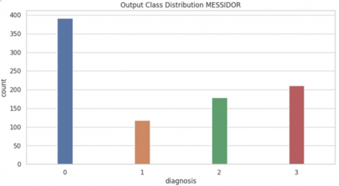
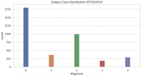
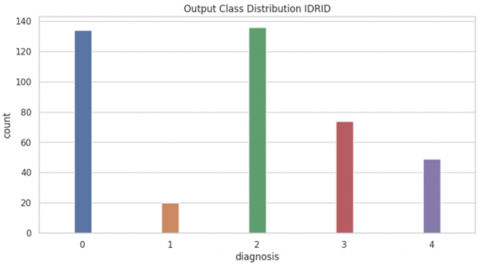
Notably, three major datasets-MESSIDOR, APTOS, and IDRID-are discussed in the following subsections. Figure 4 illustrates the difference between the data distribution in these datasets.
5.1.1 MESSIDOR
The MESSIDOR dataset contains 1,200 color fundus images in TIFF format. Initially created for assessing retinal lesion segmentation algorithms, it includes detailed annotations with diabetic retinopathy (DR) grades assigned to each image [43]. As depicted in Figure 4(a), the images are divided into four classification categories. This dataset is among the largest available and plays a crucial role in advancing computer-assisted diagnosis (CAD) systems for DR.
5.1.2 APTOS
The APTOS dataset is collected by the Indian Aravind Eye Hospital in collaboration with the Asia pacific tele-ophthalmology society (APTOS). It contains 3,662 retinal images captured using various cameras in different resolutions. It involves five classification levels (see Figure 4(b)). However, the only publicly accessible labels are the ground-truth labels. There is a notable class imbalance, with 1,805 normal retina images against 183 images that show severe non-proliferative diabetic retinopathy (NPDR) [44]. Because of the variations in imaging equipment and settings across different centers, the dataset reflects real-world inconsistencies.
(a) MESSIDOR dataset
(b) APTOS-2019 dataset
(c) IDRID dataset
Figure 4. Difference between MESSIDOR, APTOS-2019 and IDRID datasets in terms of data distribution
5.1.3 IDRID
The Indian diabetic retinopathy image dataset (IDRID) is a key resource for diabetic retinopathy research, offering 516 high-resolution retinal fundus images from diabetic patients. These images are divided into training and testing sets and come with detailed annotations indicating diabetic retinopathy (DR) severity levels and specific lesions such as microaneurysms, hemorrhages, soft exudates, and hard exudates. IDRID dataset involves five classification levels (see Figure 4(c)).
Captured with high-resolution fundus cameras, the IDRID images mirror the diversity and variability found in clinical practice, making the dataset especially valuable for creating robust models. It supports a range of applications, including DR classification, fine-grained grading, lesion detection, and segmentation, proving essential resource for the development and testing of machine learning algorithms.
Recognized and widely used in the research community, the IDRID dataset is crucial for advancing computer-assisted diagnosis (CAD) systems, which are vital for the early detection and treatment of diabetic retinopathy. Its public availability ensures global access, encouraging collaboration and speeding up progress in the field.
In summary, the comprehensive annotations and high-quality images provided by the IDRID dataset are vital for enhancing the accuracy and reliability of automated DR detection and assessment systems, establishing it as a fundamental resource in diabetic retinopathy research.
The MESSIDOR, APTOS, and IDRID datasets serve as essential resources for both research and and development in the domain of retinal ophthalmology. Indeed, these datasets enable a comprehensive evaluation and benchmarking of algorithms for detecting and classifying retinal diseases like diabetic retinopathy (DR), especially, in presence of well-annotated data and established ground-truth. They play a vital role in fostering advancements in Computer-Aided Diagnosis (CAD) systems and AI-driven solutions in ophthalmology.
5.2 Performance evaluation metrics
Given that TP (resp. FP) indicates the number of positive samples correctly predicted (resp. incorrectly predicted) and TN (resp. FN) indicates the number of negative samples correctly predicted (resp. incorrectly predicted), in his paper, we use the following main performance evaluation metrics:
5.2.1 Accuracy
Accuracy is calculated as the ratio of the number of samples that are correctly predicted to the total number of samples (see Eq. (13)).
Accuracy $=\frac{T P+T N}{T P+T N+F P+F N}$ (13)
5.2.2 Precision
Precision measures the proportion of true positive predictions (correct positive predictions) out of all positive predictions made by the model. It is calculated by Eq. (14):
Precision $=\frac{T P}{T P+F P}$ (14)
5.2.3 Recall (Sensitivity)
Recall, also known as sensitivity or true positive rate, measures the proportion of true positive predictions that are correctly identified by the model. It is calculated by Eq. (15):
Recall $=\frac{T P}{T P+F N}$ (15)
5.2.4 F1-Score
The F1-score is the harmonic mean of precision and recall, providing a single metric that balances both measures. It is calculated by Eq. (16):
$F 1-$ score $=2 \times \frac{\text { Precision × Recall }}{\text { Precision }+ \text { Recall }}$ (16)
5.2.5 Cohen’s kappa coefficient ($\boldsymbol{\kappa}$)
Cohen’s kappa coefficient ($\boldsymbol{\kappa}$) is a statistical metric used to evaluate inter-rater and intra-rater reliability [45]. Unlike a simple agreement calculation, it provides a more reliable measure by accounting for the likelihood of agreement occurring by chance. Cohen’s kappa is mathematically represented in Eq. (17):
$\kappa=\frac{p_o-p_e}{1-p_c}=1-\frac{1-p_o}{1-p_c}$ (17)
where $p_o$ denotes the observed agreement and $p_e$ represents the expected agreement. Essentially, this metric indicates how much better a classifier performs compared to random guessing based on class distribution. The formula can also be derived from the confusion matrix, as shown in Eq. (18):
$\kappa=\frac{2 \times(T P \times T N-F N \times F P)}{(T P+F P) \times(F P+T N)+(T P+F N) \times(F N+T N)}$ (18)
In this paper, we use multiple metrics, including sensitivity (Precision), specificity (Recall), accuracy (ACC), F1-score (F1), and the area under the ROC curve (AUCROC) multiple metrics, to evaluate classification performance.
To highlight the effectiveness of the ALMMo-0 methodology, we compared it with a diverse set of well-known machine learning and deep learning algorithms. These include traditional machine learning models: gaussian naïve bayes (GNB), support vector machine (SVM), K-Nearest Neighbors (KNN), random forest (RF), extra trees (ET), and logistic regression (LR). Additionally, we evaluated deep learning approaches such as deep neural networks (DNN), convolutional neural networks (CNN), and long short-term memory (LSTM) networks. The classification results obtained from these models are detailed in Tables 2-13 and visually represented in Figures 5-10.
Table 2. Precision of the different classification algorithms with MESSIDOR-2 dataset
|
Precision |
||||||||||
|
|
Ours |
GB |
SVM |
RF |
KNN |
LR |
ET |
DNN |
CNN |
LSTM |
|
None |
0.89 |
0.81 |
0.53 |
0.90 |
0.95 |
0.61 |
0.91 |
0.61 |
0.84 |
0.53 |
|
Mild DR |
0.79 |
0.20 |
0.00 |
1.00 |
0.91 |
0.29 |
1.00 |
1.00 |
0.83 |
0.00 |
|
Moderate DR |
0.86 |
0.43 |
0.00 |
0.95 |
0.92 |
0.47 |
0.96 |
0.75 |
0.62 |
0.00 |
|
Severe DR |
0.93 |
0.66 |
0.73 |
0.98 |
0.97 |
0.66 |
0.95 |
0.76 |
1.00 |
0.82 |
|
Avg |
0.88 |
0.63 |
0.41 |
0.94 |
0.95 |
0.56 |
0.94 |
0.72 |
0.83 |
0.42 |
Table 3. F1-score of the different classification algorithms with MESSIDOR-2 dataset
|
F1-Score |
||||||||||
|
|
Ours |
GB |
SVM |
RF |
KNN |
LR |
ET |
DNN |
CNN |
LSTM |
|
None |
0.92 |
0.37 |
0.68 |
0.94 |
0.95 |
0.71 |
0.95 |
0.74 |
0.86 |
0.69 |
|
Mild DR |
0.86 |
0.32 |
0.00 |
0.92 |
0.92 |
0.06 |
0.92 |
0.04 |
0.81 |
0.00 |
|
Moderate DR |
0.83 |
0.37 |
0.00 |
0.92 |
0.93 |
0.37 |
0.92 |
0.51 |
0.72 |
0.00 |
|
Severe DR |
0.86 |
0.31 |
0.61 |
0.94 |
0.96 |
0.61 |
0.93 |
0.73 |
0.78 |
0.68 |
|
Avg |
0.88 |
0.40 |
0.45 |
0.94 |
0.95 |
0.45 |
0.94 |
0.60 |
0.80 |
0.47 |
Table 4. Recall of the different classification algorithms with MESSIDOR-2 dataset
|
Recall |
||||||||||
|
|
Ours |
GB |
SVM |
RF |
KNN |
LR |
ET |
DNN |
CNN |
LSTM |
|
None |
0.95 |
0.24 |
0.96 |
0.99 |
0.95 |
0.85 |
0.99 |
0.92 |
0.87 |
0.98 |
|
Mild DR |
0.95 |
0.93 |
0.00 |
0.86 |
0.93 |
0.04 |
0.86 |
0.02 |
0.79 |
0.00 |
|
Moderate DR |
0.79 |
0.32 |
0.00 |
0.90 |
0.94 |
0.31 |
0.89 |
0.39 |
0.84 |
0.00 |
|
Severe DR |
0.80 |
0.41 |
0.52 |
0.91 |
0.94 |
0.63 |
0.92 |
0.70 |
0.63 |
0.58 |
|
Avg |
0.88 |
0.38 |
0.56 |
0.94 |
0.95 |
0.60 |
0.94 |
0.66 |
0.80 |
0.58 |
Table 5. Performance of the different classification algorithms with MESSIDOR-2 dataset
|
All Metrics |
||||||
|
|
Precision |
Recall |
ACC |
F1-score |
ROC |
k |
|
KNN |
0.95 |
0.95 |
0.95 |
0.95 |
0.89 |
0.92 |
|
GB |
0.63 |
0.38 |
0.38 |
0.40 |
0.71 |
0.23 |
|
ET |
0.94 |
0.94 |
0.94 |
0.94 |
0.98 |
0.90 |
|
RF |
0.94 |
0.94 |
0.94 |
0.94 |
0.98 |
0.90 |
|
SVM |
0.45 |
0.56 |
0.56 |
0.45 |
0.79 |
0.24 |
|
LR |
0.55 |
0.60 |
0.60 |
0.55 |
0.80 |
0.36 |
|
CNN |
0.83 |
0.80 |
0.80 |
0.80 |
0.95 |
0.71 |
|
DNN |
0.72 |
0.66 |
0.65 |
0.60 |
0.84 |
0.44 |
|
LSTM |
0.42 |
0.58 |
0.57 |
0.47 |
0.70 |
0.27 |
|
Ours |
0.98 |
0.88 |
0.87 |
0.87 |
0.88 |
0.82 |
Table 6. F1-score of the different classification algorithms with IDRID dataset
|
F1-score |
||||||||||
|
|
Ours |
GB |
SVM |
RF |
KNN |
LR |
ET |
DNN |
CNN |
LSTM |
|
No DR |
0.98 |
0.58 |
0.92 |
0.99 |
1.00 |
0.94 |
0.99 |
0.94 |
0.86 |
0.82 |
|
Mild |
0.89 |
0.28 |
0.07 |
0.94 |
0.97 |
0.48 |
0.94 |
0.52 |
0.81 |
0.00 |
|
Moderate |
0.98 |
0.18 |
0.68 |
0.96 |
0.98 |
0.72 |
0.95 |
0.72 |
0.72 |
0.58 |
|
Severe |
0.96 |
0.41 |
0.00 |
0.93 |
0.96 |
0.35 |
0.92 |
0.59 |
0.78 |
0.36 |
|
Proliferative DR |
0,96 |
0.38 |
0.01 |
0.93 |
0.96 |
0.38 |
0.93 |
0.57 |
0.99 |
0.07 |
|
Avg |
0.97 |
0.42 |
0.64 |
0.97 |
0.98 |
0.75 |
0.97 |
0.79 |
0.81 |
0.58 |
Table 7. Precision of the different classification algorithms with IDRID dataset
|
Precision |
||||||||||
|
|
Ours |
GB |
SVM |
RF |
KNN |
LR |
ET |
DNN |
CNN |
LSTM |
|
No DR |
0.97 |
0.92 |
0.87 |
0.99 |
1.00 |
0.90 |
0.98 |
0.98 |
0.84 |
0.99 |
|
Mild |
1.00 |
0.16 |
0.62 |
0.97 |
0.96 |
0.67 |
0.97 |
0.58 |
0.83 |
0.00 |
|
Moderate |
0.99 |
0.70 |
0.55 |
0.93 |
0.98 |
0.64 |
0.93 |
0.64 |
0.62 |
0.42 |
|
Severe |
0.93 |
0.38 |
0.00 |
0.98 |
0.97 |
0.74 |
0.97 |
0.60 |
1.00 |
0.42 |
|
Proliferative DR |
1.00 |
0.36 |
1.00 |
0.98 |
0.96 |
0.55 |
0.97 |
0.67 |
0.99 |
0.75 |
|
Avg |
0.97 |
0.70 |
0.72 |
0.97 |
0.98 |
0.77 |
0.97 |
0.80 |
0.83 |
0.69 |
Table 8. Recall of the different classification algorithms with IDRID dataset
|
Recall |
||||||||||
|
|
Ours |
GB |
SVM |
RF |
KNN |
LR |
ET |
DNN |
CNN |
LSTM |
|
No DR |
1.00 |
0.43 |
0.98 |
1.00 |
0.99 |
0.98 |
0.99 |
0.90 |
0.87 |
0.70 |
|
Mild |
0.80 |
0.88 |
0.04 |
0.92 |
0.98 |
0.38 |
0.91 |
0.47 |
0.79 |
0.00 |
|
Moderate |
0.97 |
0.11 |
0.90 |
0.98 |
0.98 |
0.83 |
0.97 |
0.83 |
0.84 |
0.95 |
|
Severe |
1.00 |
0.45 |
0.00 |
0.89 |
0.94 |
0.23 |
0.88 |
0.59 |
0.63 |
0.32 |
|
Proliferative DR |
0.93 |
0.41 |
0.01 |
0.89 |
0.96 |
0.29 |
0.89 |
0.49 |
0.99 |
0.04 |
|
Avg |
0.97 |
0.39 |
0.72 |
0.97 |
0.98 |
0.78 |
0.97 |
0.79 |
0.80 |
0.62 |
Table 9. Performance of the different classification algorithms with IDRID dataset
|
All metrics |
||||||
|
|
Precision |
Recall |
ACC |
F1-Score |
ROC |
k |
|
KNN |
0.98 |
0.98 |
0.98 |
0.98 |
0.95 |
0.98 |
|
GB |
0.50 |
0.39 |
0.39 |
0.42 |
0.51 |
0.54 |
|
ET |
0.97 |
0.97 |
0.96 |
0.97 |
0.96 |
0.97 |
|
RF |
0.97 |
0.97 |
0.97 |
0.97 |
0.96 |
0.97 |
|
SVM |
0.72 |
0.72 |
0.72 |
0.64 |
0.70 |
0.73 |
|
LR |
0.77 |
0.78 |
0.78 |
0.75 |
0.75 |
0.80 |
|
CNN |
0.83 |
0.80 |
0.80 |
0.80 |
0.95 |
0.71 |
|
DNN |
0.80 |
0.79 |
0.79 |
0.79 |
0.94 |
0.68 |
|
LSTM |
0.69 |
0.62 |
0.61 |
0.58 |
0.86 |
0.42 |
|
Ours |
0.98 |
0.96 |
0.97 |
0.97 |
0.99 |
0.96 |
Table 10. F1-score of the different classification algorithms with APTOS-2019 dataset
|
F1-Score |
||||||||||
|
|
Ours |
GB |
SVM |
RF |
KNN |
LR |
ET |
DNN |
CNN |
LSTM |
|
No DR |
0.98 |
0.56 |
0.90 |
0.99 |
1.00 |
0.94 |
0.99 |
0.87 |
0.87 |
0.76 |
|
Mild |
0.86 |
0.28 |
0.10 |
0.94 |
0.96 |
0.48 |
0.94 |
0.99 |
0.29 |
0.00 |
|
Moderate |
0.92 |
0.18 |
0.70 |
0.96 |
0.98 |
0.72 |
0.95 |
0.81 |
0.81 |
0.58 |
|
Severe |
0.82 |
0.41 |
0.00 |
0.93 |
0.95 |
0.35 |
0.92 |
0.81 |
0.72 |
0.30 |
|
Proliferative DR |
0.85 |
0.40 |
0.10 |
0.93 |
0.96 |
0.38 |
0.93 |
0.69 |
0.77 |
0.00 |
|
Avg |
0.93 |
0.42 |
0.64 |
0.91 |
0.98 |
0.75 |
0.97 |
0.79 |
0.80 |
0.49 |
Table 11. Precision of the different classification algorithms with APTOS-2019 dataset
|
Precision |
||||||||||
|
|
Ours |
GB |
SVM |
RF |
KNN |
LR |
ET |
DNN |
CNN |
LSTM |
|
No DR |
0.98 |
0.92 |
0.87 |
0.99 |
1.00 |
0.90 |
0.98 |
0.83 |
0.98 |
0.73 |
|
Mild |
0.86 |
0.16 |
0.62 |
0.97 |
0.96 |
0.67 |
0.97 |
1.00 |
0.67 |
0.00 |
|
Moderate |
0.89 |
0.70 |
0.55 |
0.93 |
0.98 |
0.64 |
0.93 |
0.75 |
0.70 |
0.46 |
|
Severe |
0.87 |
0.38 |
0.00 |
0.98 |
0.97 |
0.74 |
0.97 |
0.84 |
0.96 |
0.50 |
|
Proliferative DR |
0.90 |
0.36 |
1.00 |
0.98 |
0.96 |
0.55 |
0.79 |
0.65 |
0.99 |
0.00 |
|
Avg |
0.90 |
0.70 |
0.72 |
0.97 |
0.98 |
0.77 |
0.97 |
0.81 |
0.84 |
0.49 |
Table 12. Recall of the different classification algorithms with APTOS-2019 dataset
|
Recall |
||||||||||
|
|
Ours |
GB |
SVM |
RF |
KNN |
LR |
ET |
DNN |
CNN |
LSTM |
|
No DR |
0.98 |
0.43 |
0.98 |
1.00 |
0.99 |
0.98 |
0.99 |
0.91 |
0.78 |
0.79 |
|
Mild |
0.86 |
0.88 |
0.04 |
0.92 |
0.98 |
0.38 |
0.91 |
0.17 |
0.67 |
0.00 |
|
Moderate |
0.95 |
0.11 |
0.90 |
0.98 |
0.98 |
0.83 |
0.97 |
0.87 |
0.96 |
0.78 |
|
Severe |
0.77 |
0.45 |
0.00 |
0.89 |
0.94 |
0.23 |
0.88 |
0.79 |
0.57 |
0.21 |
|
Proliferative DR |
0.88 |
0.41 |
0.01 |
0.89 |
0.96 |
0.61 |
0.89 |
0.94 |
0.99 |
0.00 |
|
Avg |
0.93 |
0.39 |
0.72 |
0.97 |
0.98 |
0.78 |
0.97 |
0.80 |
0.80 |
0.55 |
Table 13. Performance of the different classification algorithms with APTOS-2019 dataset
|
All Metrics |
||||||
|
|
Precision |
Recall |
ACC |
F1-score |
ROC |
k |
|
KNN |
0.98 |
0.98 |
0.98 |
0.98 |
0.95 |
0.98 |
|
GB |
0.50 |
0.39 |
0.39 |
0.42 |
0.51 |
0.54 |
|
ET |
0.97 |
0.97 |
0.96 |
0.97 |
0.96 |
0.97 |
|
RF |
0.97 |
0.97 |
0.97 |
0.97 |
0.96 |
0.97 |
|
SVM |
0.72 |
0.72 |
0.72 |
0.64 |
0.70 |
0.73 |
|
LR |
0.77 |
0.78 |
0.78 |
0.75 |
0.75 |
0.80 |
|
CNN |
0.84 |
0.80 |
0.79 |
0.80 |
0.97 |
0.72 |
|
DNN |
0.81 |
0.80 |
0.81 |
0.79 |
0.97 |
0.72 |
|
LSTM |
0.49 |
0.55 |
0.54 |
0.49 |
0.81 |
0.53 |
|
Ours |
0.93 |
0.92 |
0.93 |
0.93 |
0.93 |
0.89 |
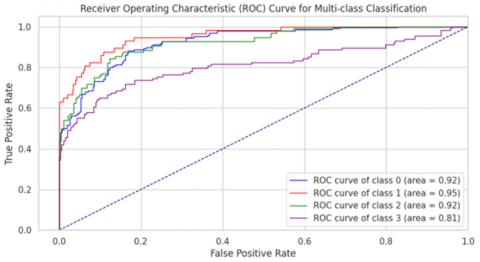
Figure 5. The multiclass receiver operating characteristic for MESSIDOR-2 dataset
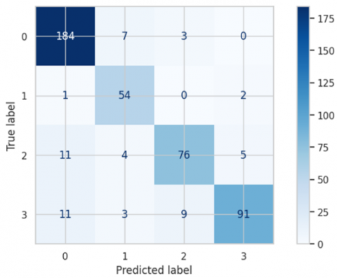
Figure 6. Confusion Matrix for MESSIDOR-2
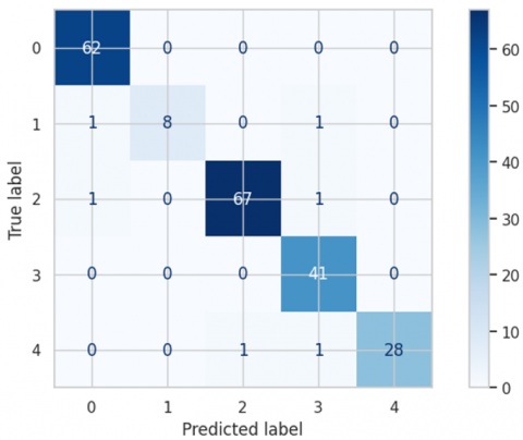
Figure 7. Confusion Matrix for IDRID dataset
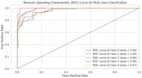
Figure 8. The multiclass receiver operating characteristic for IDRID dataset
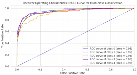
Figure 9. The multiclass receiver operating characteristic for APTOS-2019 dataset
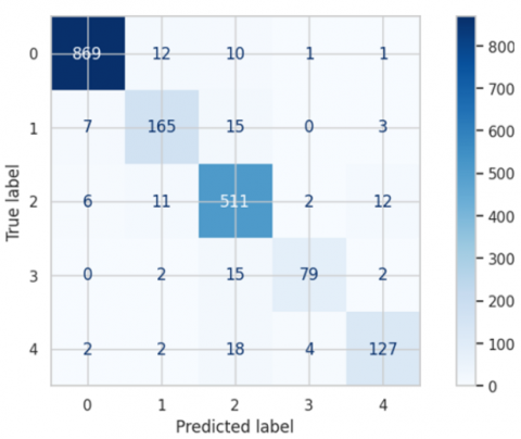
Figure 10. Confusion Matrix for APTOS-2019
5.3 Results for MESSIDOR-2 dataset
The ALMOO-0 model was trained on the MESSIDOR-2 dataset, achieving outstanding performance across all evaluated metrics. As shown in Table 5, ALMOO-0 reached average scores of 98% for precision, 88% for recall, 87% for F1-score, 87% for accuracy, 88% for ROC-AUC, and 82% for Cohen’s κ.
Among the evaluated models, the KNN algorithm delivered the second-best overall performance, with 95% precision, 95% recall, 95% accuracy, and a ROC-AUC of 89%. Tree-based ensemble methods such as RF and ET also performed strongly, each scoring 94% in precision, recall, accuracy, and F1-score, along with a ROC-AUC of 98%. In contrast, traditional algorithms like GB and SVM achieved notably lower results, with average precision values of 63% and 45%, respectively.
The ALMOO-0 model demonstrated excellent precision across all DR categories (Table 2), with particularly high values for Severe DR (0.93) and None (0.89). Its F1-scores (Table 3) were also consistently high, achieving 0.92 for None and 0.86 for Mild DR, and an overall average of 0.88. For recall (Table 4), ALMOO-0 maintained balanced sensitivity across all classes, with 0.95 for None and 0.95 for Mild DR.
5.4 Results for IDRID dataset
The ALMMo-0 model was rigorously trained on the IDRID dataset, leading to exceptional evaluation results. As detailed in Table 9, the model achieved outstanding performance metrics, with an average precision, recall, F1-score, and accuracy rate all reaching 99.7%. In addition to these metrics, the ALMMo-0 model delivered remarkable results in terms of the area under the curve (AUC), with an average AUC of 99.8%. The AUC values for individual classes are visually represented in Figure 8, demonstrating excellent performance across all categories. AUC values exceeded 95% for all classes, highlighting the robustness of the proposed approach in successfully detecting all classes of diabetic retinopathy (DR).
5.5 Results for APTOS-2019 dataset
The APTOS (Asia Pacific Tele-Ophthalmology Society) dataset is a significant resource used in the development of machine learning models for detecting diabetic retinopathy from retinal images. This dataset was created as part of a Kaggle competition in 2019 and contains 3,662 high-resolution fundus images, each annotated by medical experts with one of five severity levels of diabetic retinopathy, ranging from no retinopathy to proliferative diabetic retinopathy. The APTOS dataset is particularly valuable due to its diversity in image quality and variation in retinal conditions, which provides a challenging environment for developing robust and generalizable models.
This research paper introduces a novel method for efficient diabetic retinopathy detection using the Adaptive learning multimodal optimization-oriented (ALMMo-0) model. Unlike traditional deep learning techniques, this approach offers a transparent and interpretable internal architecture. The ALMMo-0 model not only ensures excellent accuracy, but also significantly improves training efficiency and explainability.
Training Efficiency. One of the key advantages of the ALMMo-0 model is its efficiency in terms of computational resources and training time. Unlike conventional deep learning methods that often require powerful GPUs and extended training periods, ALMMo-0 operates effectively with minimal computational demands.
Prototype-Based Architecture. The ALMMo-0 architecture is built on a prototype-based framework, leveraging real training data samples that correspond to local maxima in the data distribution. The resulting prototypes capture characteristic data points and density patterns, serving as the foundation for a generative model expressed in a closed-form solution. As a result, the model operates without requiring user defined thresholds, parameters, or manual tuning, making it fully data-driven and systematically derived from the training set.
Harmonized Learning and Reasoning. ALMMo-0 combines learning and reasoning in a non-parametric, non-iterative and cohesive approach, improving both efficiency and interpretability. This approach provides a clear and understandable classifier that is easily interpretable by human users.
Outstanding Performance. Our empirical findings indicate that the ALMMo-0 model outperforms leading deep learning models, such as VGG-VD-16, in terms of training efficiency, accuracy a well as clarity of its decision-making process.
While the results of our study are promising, we recognize certain limitations that must be addressed to broaden the model’s applicability. The datasets used, such as MESSIDOR-2, APTOS-2019, and IDRID, may not fully represent the geographic and demographic diversity required for global generalizability. Despite careful preprocessing, image quality variability remains an issue, and the datasets are primarily focused on diabetic retinopathy and related conditions. Additionally, the model’s interpretability for clinicians, particularly in fast-paced clinical environments, requires further validation.
To overcome these challenges, future research will focus on acquiring more diverse datasets that encompass a broader range of demographics and retinal conditions. We will also explore advanced preprocessing and augmentation techniques, along with adaptive learning strategies, to enhance the model’s robustness. Pilot studies in various clinical settings will be conducted to validate the model’s performance and gather feedback for improving its integration into healthcare systems. Developing more intuitive explanation interfaces and interactive training modules for clinicians will be crucial for ensuring the model’s practical utility.
Our assumptions regarding the effectiveness of preprocessing techniques, the representativeness of the datasets, and the clinical relevance of the model’s explanations require further empirical validation. Future research will explore adaptive learning methods for minimal intervention updates and develop advanced monitoring tools for deeper performance insights. By addressing these limitations and pursuing these future directions, we aim to create a comprehensive and reliable model suitable for diverse clinical applications.
In future work, we aim to enhance the generalizability and clinical reliability of our approach through two main directions. First, we will integrate datasets from diverse geographic and clinical sources—or collect new ones—to reduce dataset bias and better represent global retinal variations. Second, we plan to collaborate with medical professionals to validate the system’s explainability by extracting and visualizing the fuzzy rules triggered during each diagnostic decision. This will provide clinicians with transparent insights into the model’s reasoning, supporting the development of a more interpretable and trustworthy diagnostic support system.
[1] Esteva, A., Kuprel, B., Novoa, R.A., Ko, J., Swetter, S.M., Blau, H.M., Thrun, S. (2017). Dermatologist-level classification of skin cancer with deep neural networks. Nature, 542(7639): 115-118. https://doi.org/10.1038/nature21056
[2] Litjens, G., Kooi, T., Bejnordi, B.E., Setio, A.A.A., Ciompi, F., Ghafoorian, M., Sánchez, C.I. (2017). A survey on deep learning in medical image analysis. Medical Image Analysis, 42: 60-88. https://doi.org/10.1016/j.media.2017.07.005
[3] Janowczyk, A., Madabhushi, A. (2016). Deep learning for digital pathology image analysis: A comprehensive tutorial with selected use cases. Journal of Pathology Informatics, 7(1): 29. https://doi.org/10.4103/2153-3539.186902
[4] Hussein, A.K. (2025). Enhancing diabetic retinopathy detection with weighted sum ensemble models. Ingénierie des Systèmes d’Information, 30(2): 483-493. https://doi.org/10.18280/isi.300220
[5] Sanamdikar, S.T., Patil, S.A., Patil, D.O., Borawake, M.P. (2023). Enhanced detection of Diabetic Retinopathy using ensemble machine learning: A comparative study. Ingénierie des Systèmes d’Information, 28(6): 1663-1668. https://doi.org/10.18280/isi.280624
[6] Shorten, C., Khoshgoftaar, T.M. (2019). A survey on image data augmentation for deep learning. Journal of Big Data, 6(1): 1-48. https://doi.org/10.1186/s40537-019-0197-0
[7] Atwany, M.Z., Sahyoun, A., Yaqub, M. (2022). Deep learning techniques for diabetic retinopathy classification: A survey. IEEE Access, 10: 28642-28655. https://doi.org/10.1109/ACCESS.2022.3157632
[8] Angelov, P., Gu, X. (2017). Autonomous learning multi-model classifier of 0-order (ALMMo-0). In 2017 Evolving and Adaptive Intelligent Systems (EAIS), Ljubljana, Slovenia, pp. 1-7. https://doi.org/10.1109/EAIS.2017.7954832
[9] Santos, F., Sousa, J.M., Vieira, S.M. (2021). A new approach to ALMMo-0 Classifiers: A trade-off between accuracy and complexity. In 2021 IEEE International Conference on Fuzzy Systems (FUZZ-IEEE), Luxembourg, Luxembourg, pp. 1-6. https://doi.org/10.1109/FUZZ45933.2021.9494579
[10] Santos, F., Ventura, R., Sousa, J.M., Vieira, S.M. (2022). First-order autonomous learning multi-model systems for multiclass classification tasks. In 2022 IEEE International Conference on Fuzzy Systems (FUZZ-IEEE), Padua, Italy, pp. 1-6. https://doi.org/10.1109/FUZZ-IEEE55066.2022.9882593
[11] Mecili, O., Barkat, H., Nouioua, F., Attia, A., Akhrouf, S. (2024). An efficient explainable deep neural network classifier for diabetic retinopathy detection. International Journal of Computers and Applications, 46(9): 795-810. https://doi.org/10.1080/1206212X.2024.2389342
[12] Gargeya, R., Leng, T. (2017). Automated identification of diabetic retinopathy using deep learning. Ophthalmology, 124(7): 962-969. https://doi.org/10.1016/j.ophtha.2017.02.008
[13] Thanikachalam, V., Kabilan, K., Erramchetty, S.K. (2024). Optimized deep CNN for detection and classification of diabetic retinopathy and diabetic macular edema. BMC Medical Imaging, 24(1): 227. https://doi.org/10.1186/s12880-024-01406-1
[14] Ainapur, S.S., Patil, V. (2024). A novel automated system for early diabetic retinopathy detection and severity classification. Journal of Chemometrics, 38(11): e3593. https://doi.org/10.1002/cem.3593
[15] Le, D., Alam, M., Yao, C.K., Lim, J.I., Hsieh, Y.T., Chan, R.V., Yao, X. (2020). Transfer learning for automated OCTA detection of diabetic retinopathy. Translational Vision Science & Technology, 9(2): 35-35. https://doi.org/10.1167/tvst.9.2.35
[16] Bodapati, J.D., Naralasetti, V., Shareef, S.N., Hakak, S., Bilal, M., Maddikunta, P.K.R., Jo, O. (2020). Blended multi-modal deep convnet features for diabetic retinopathy severity prediction. Electronics, 9(6): 914. https://doi.org/10.3390/electronics9060914
[17] Bhardwaj, C., Jain, S., Sood, M. (2021). Transfer learning based robust automatic detection system for diabetic retinopathy grading. Neural Computing and Applications, 33(20): 13999-14019. https://doi.org/10.1007/s00521-021-06042-2
[18] Pour, A.M., Seyedarabi, H., Jahromi, S.H.A., Javadzadeh, A. (2020). Automatic detection and monitoring of diabetic retinopathy using efficient convolutional neural networks and contrast limited adaptive histogram equalization. IEEE Access, 8: 136668-136673. https://doi.org/10.1109/ACCESS.2020.3005044
[19] Jena, P.K., Khuntia, B., Palai, C., Nayak, M., Mishra, T.K., Mohanty, S.N. (2023). A novel approach for diabetic retinopathy screening using asymmetric deep learning features. Big Data and Cognitive Computing, 7(1): 25. https://doi.org/10.3390/bdcc7010025
[20] Nur-A-Alam, M., Nasir, M.M.K., Ahsan, M., Based, M.A., Haider, J., Palani, S. (2023). A faster RCNN-based diabetic retinopathy detection method using fused features from retina images. IEEE Access, 11: 124331-124349. https://doi.org/10.1109/ACCESS.2023.3330104
[21] İncir, R., Bozkurt, F. (2024). A study on the segmentation and classification of diabetic retinopathy images using the k-means clustering method. In 2024 32nd Signal Processing and Communications Applications Conference (SIU), Mersin, Turkiye, pp. 1-4. https://doi.org/10.1109/SIU61531.2024.10600987
[22] Omer, H.K. (2024). Diabetic retinopathy detection using Bilayered Neural Network classification model with resubstitution validation. MethodsX, 12: 102705. https://doi.org/10.1016/j.mex.2024.102705
[23] Akhtar, S., Aftab, S., Kousar, S., Rehman, A., Ahmad, M., Saeed, A.Q. (2024). A severity grading framework for diabetic retinopathy detection using transfer learning. In 2024 International Conference on Decision Aid Sciences and Applications (DASA), Manama, Bahrain, pp. 1-5. https://doi.org/10.1109/DASA63652.2024.10836441
[24] Manasa, G.R., Anchan, A., Santhosh, T., Hemashree, H.C., Pinnapati, S., Shetty, S.S. (2024). Diabetic retinopathy detection from retina image using machine learning. In 2024 IEEE International Conference on Distributed Computing, VLSI, Electrical Circuits and Robotics (DISCOVER), Mangalore, India, pp. 279-285. https://doi.org/10.1109/DISCOVER62353.2024.10750625
[25] Costaner, L., Lisnawita, L., Guntoro, G., Abdullah, A. (2024). Feature extraction analysis for diabetic retinopathy detection using machine learning techniques. SISTEMASI, 13(5): 2268-2276. https://doi.org/10.32520/stmsi.v13i5.4600
[26] Li, Z., Huang, Y. (2023). Vision transformer for diabetic retinopathy grading using fundus images. IEEE Transactions on Medical Imaging.
[27] Dosovitskiy, A. (2020). An image is worth 16x16 words: Transformers for image recognition at scale. arXiv preprint arXiv:2010.11929.
[28] Xu, Y., Wang, T. (2024). Swin transformer-based hierarchical network for diabetic retinopathy classification. Computers in Biology and Medicine.
[29] Koh, P.W., Nguyen, T., Tang, Y.S., Mussmann, S., Pierson, E., Kim, B., Liang, P. (2020). Concept bottleneck models. In International Conference on Machine Learning, pp. 5338-5348. https://ui.adsabs.harvard.edu/link_gateway/2020arXiv200704612K/doi:10.48550/arXiv.2007.04612.
[30] Lage, I., Ross, A.S., Kim, B., Gershman, S.J., Doshi-Velez, F. (2018). Human-in-the-loop interpretability prior. In Proceedings of the 32nd International Conference on Neural Information Processing Systems, Canada, pp. 10180-10189. https://doi.org/10.48550/arXiv.1805.11571
[31] Barredo Arrieta, A., Díaz-Rodríguez, N., Del Ser, J., Bennetot, A., Tabik, S., Barbado, A., Herrera, F. (2020). Explainable Artificial Intelligence (XAI): Concepts, taxonomies, opportunities, and challenges toward responsible AI. Information Fusion, 58: 82-115. https://doi.org/10.1016/j.inffus.2019.12.012
[32] Gunning, D., Stefik, M., Choi, J., Miller, T., Stumpf, S., Yang, G.Z. (2019). XAI-Explainable artificial intelligence. Science robotics, 4(37): eaay7120. https://doi.org/10.1126/scirobotics.aay7120
[33] Grassmann, F., Mengelkamp, J., Brandl, C., Harsch, S., Zimmermann, M.E., Linkohr, B., Weber, B.H. (2018). A deep learning algorithm for prediction of age-related eye disease study severity scale for age-related macular degeneration from color fundus photography. Ophthalmology, 125(9): 1410-1420. https://doi.org/10.1016/j.ophtha.2018.02.037
[34] Goodfellow, I.J., Pouget-Abadie, J., Mirza, M., Xu, B., Warde-Farley, D., Ozair, S., Bengio, Y. (2014). Generative adversarial nets. Advances in Neural Information Processing Systems, 27: 139-144.
[35] Gulshan, V., Peng, L., Coram, M., Stumpe, M.C., Wu, D., Narayanaswamy, A., Webster, D.R. (2016). Development and validation of a deep learning algorithm for detection of diabetic retinopathy in retinal fundus photographs. Jama, 316(22): 2402-2410. https://doi.org/10.1001/jama.2016.17216
[36] Abràmoff, M.D., Lou, Y., Erginay, A., Clarida, W., Amelon, R., Folk, J.C., Niemeijer, M. (2016). Improved automated detection of diabetic retinopathy on a publicly available dataset through integration of deep learning. Investigative Ophthalmology & Visual Science, 57(13): 5200-5206. https://doi.org/10.1167/iovs.16-19964
[37] Angelov, P.P., Gu, X., Principe, J.C. (2017). Autonomous learning multimodel systems from data streams. IEEE Transactions on Fuzzy Systems, 26(4): 2213-2224. https://doi.org/10.1109/TFUZZ.2017.2769039
[38] Reza, A.M. (2004). Realization of the contrast limited adaptive histogram equalization (CLAHE) for real-time image enhancement. Journal of VLSI Signal Processing Systems for Signal, Image and Video Technology, 38(1): 35-44. https://doi.org/10.1023/B:VLSI.0000028532.53893.82
[39] Mamdani, E.H., Assilian, S. (1975). An experiment in linguistic synthesis with a fuzzy logic controller. International Journal of Man-machine Studies, 7(1): 1-13. https://doi.org/10.1016/S0020-7373(75)80002-2
[40] Zadeh, L.A. (1973). Outline of a new approach to the analysis of complex systems and decision processes. IEEE Transactions on Systems, Man, and Cybernetics, 3(1): 28-44. https://doi.org/10.1109/TSMC.1973.5408575
[41] Takagi, T., Sugeno, M. (1985). Fuzzy identification of systems and its applications to modeling and control. IEEE Transactions on Systems, Man, and Cybernetics, 15(1): 116-132. https://doi.org/10.1109/TSMC.1985.6313399
[42] Okabe, A., Boots, B., Sugihara, K., Chiu, S.N. (1999). Spatial Tessellations: Concepts and Applications of Voronoi Diagrams. John Wiley & Sons.
[43] Decencière, E., Zhang, X., Cazuguel, G., Lay, B., et al. (2014). Feedback on a publicly distributed image database: The Messidor database. Image Analysis & Stereology, 33(3): 231-234. https://doi.org/10.5566/ias.1155
[44] Alyoubi, W.L., Abulkhair, M.F., Shalash, W.M. (2021). Diabetic retinopathy fundus image classification and lesions localization system using deep learning. Sensors, 21(11): 3704. https://doi.org/10.3390/s21113704
[45] Cohen, J. (1960). A coefficient of agreement for nominal scales. Educational and Psychological Measurement, 20(1): 37-46. https://doi.org/10.1177/001316446002000104