Ngoc Thai Huynh![]() | Chi Bao Phan
| Chi Bao Phan![]() | Trieu Khoa Nguyen*
| Trieu Khoa Nguyen*![]() | Minh Tuan Nguyen
| Minh Tuan Nguyen![]() | Vu Hai Le
| Vu Hai Le![]() | Minh Hung Vu
| Minh Hung Vu![]() | Quoc Manh Nguyen
| Quoc Manh Nguyen![]()
© 2025 The authors. This article is published by IIETA and is licensed under the CC BY 4.0 license (http://creativecommons.org/licenses/by/4.0/).
OPEN ACCESS
Achieving high displacement amplification in compliant mechanisms using flexural hinges is a challenging task in precision engineering, especially when multiple performance criteria must be considered. This study proposes an integrated optimization approach that combines the Simple Additive Weighting (SAW) method with Finite Element Method (FEM) analysis to enhance the performance of elastic amplifier mechanisms. A total of 27 design variants were created using Minitab software and modeled in Inventor with circular flexural hinges. FEM simulations were conducted to evaluate stress and displacement in each design. The SAW method was applied to rank the designs based on multi-criteria decision-making, and the results were further validated using Taguchi analysis and 3D surface plots. The optimized amplifier mechanism achieved a displacement amplification ratio (DAR) of 67.237, with less than 3% deviation between predicted and simulated results, indicating high accuracy and consistency. This outcome demonstrates that the proposed method effectively balances the trade-offs between structural stiffness and amplification efficiency. The integration of SAW and FEM provides a practical and reliable framework for optimizing compliant mechanisms, making it highly applicable to microscale actuators and precision motion systems where both accuracy and amplification are critical.
compliant mechanism amplifier, circular flexure hinge, leaf flexure hinge, FEM-based stress-displacement analysis, Simple Additive Weighting (SAW) method, MEREC method, Taguchi method, displacement amplification ratio (DAR)
Compliant mechanisms, which transfer motion and force through elastic deformation rather than traditional rigid-body joints, have gained increasing attention in micro/nano-scale applications due to their advantages in miniaturization, precision, and reduced assembly complexity. In fields such as ultra-precision machining, MEMS devices, and biomedical systems, the demand for high-performance compliant structures continues to grow.
One of the key components in compliant mechanisms was the flexure hinge, particularly the lever-type bending hinge, which allows for significant displacement amplification. However, designing such mechanisms to achieve both large displacement and high stiffness remains a challenge due to the inherent trade-offs between flexibility, strength, and structural stability. Traditional optimization approaches, while effective to some extent, often require high computational effort or lack general applicability to complex geometries.
In this context, the dimensional asymmetric rectangular (DAR) hinge structure offers promising potential due to its geometric adaptability and ability to achieve amplified motion. Yet, studies on the optimization of DAR hinges remain limited, especially in terms of multi-criteria performance involving displacement, stiffness, and reliability under real-world conditions.
To address this gap, the present study proposes a novel optimization framework that combines the Simple Additive Weighting (SAW) method, Taguchi experimental design, and Finite Element Method (FEM) analysis. This hybrid approach enables efficient multi-objective optimization while ensuring both computational efficiency and experimental reliability.
The aim of this investigation was to improve the displacement amplification characteristics of compliant mechanisms through systematic analysis and optimization of DAR hinges. The novelty lay in integrating decision-making techniques (SAW), design of experiments (Taguchi), and computational modeling (FEM) to derive a practical and reliable solution.
Building upon this motivation, the following section reviews existing research related to displacement amplification, stiffness modeling, and experimental validation of various compliant mechanism designs.
The displacement amplification of the lever-type bending hinge is due to the rotation center of the bending hinge [1]. Experimental testing confirmed the results with an error of 2.49% which is comparable to FEM. A stiffness model [2] is proposed to adjust the stiffness of the compliance mechanism. The experimental results and the finite element method are consistent with the proposed model. Fast tool controller [3] proposed to improve the performance of ultra-precision machining. In order to improve the displacement amplification of the gripper, a shape memory alloy was proposed with the help of a pseudo-rigid body model. The experiment and results of the proposed model achieved a bearing capacity of 0.152 to 0.381 N. Column bending test and four-point bending test [4] were performed to test the deflection. The test results showed that the storage deflection ranged from 0.4 mm to 1 mm. The hybrid bending hinge was designed from elliptical and hyperbolic shapes [5]. The performance of the hybrid bending hinge is better than elliptical bending hinge and the hyperbolic bending hinge. New design of knurled bending hinge [6] designed by changing the elliptical cross-section. Experiments have confirmed the performance of the new model. Working plane of the elastic positioning platform with two degrees of freedom (DOF) 28.7 µm × 27.62 µm [7] obtained by experimental testing. This result is consistent with the finite element model. Two-DOF elastic positioning platform [8] The working range of 28.27 µm × 27.62 µm was achieved through actual testing. The results are in good agreement with the finite element analysis results. The stiffness model and finite element model [9] were applied to achieve minimal parasitic displacement of the XYZ stage decoupled from the bending-based motion with a quasi-symmetric 3-Prism-Prism-Prism structure. The experimental results were validated against the results of the models. A compound amplifier [10] was applied to improve the working range of the gripper elastic mechanism. The experimental results obtained DAR 34.5 times higher than the finite element analysis results in ANSYS. Experiments and finite element models were applied to determine the DAR of a single-stage nonlinear design elastic orthogonal displacement amplifier [11]. To address low amplification ratios in precision positioning systems [12], a new Z-shaped flexure hinge (ZFH) and a 2DOF XY platform using this hinge and bridge-type mechanisms for secondary amplification were proposed. Static modeling and simulations confirm improved performance, with stiffness and amplification errors under 7% and a 50.70% enhancement in ZFH efficiency. A prototype was built, and experimental results validated the design's effectiveness. A compound lever-based compliant mechanism [13] was optimized to improve MEMS accelerometer sensitivity. Using the pseudo-rigid body model and FEA, the design achieves higher displacement and natural frequency with a smaller proof mass, outperforming conventional designs in sensitivity and linearity. A piezoelectric in-plane resonator with a symmetrical oblique-beam amplification structure [14] was developed and analyzed. An analytical model was created and optimized to maximize horizontal displacement. Simulations validated the model and identified the optimal mode with strong in-plane motion and minimal out-of-plane displacement. The fabricated device achieved a 7.71 μm displacement at 16.57 kHz under a 20 Vp-p signal. A microthermal actuator with L-shaped levers and half-bridge amplification [15] was fabricated and tested, achieving 3.55 × displacement and 19 μm actuation at 15 V. Temperature-dependent simulations matched experiments, and a new performance index showed the device outperforms others in efficiency, with a top PEI of 0.0021 μm/mm²/K/V at 10 V. A piezoelectric-driven three-axis compliant gripper [16] was developed for precise in-plane and out-of-plane manipulation of small rigid objects. It uses two piezo actuators for in-plane motion and a piezo sheet for out-of-plane movement. Theoretical models, supported by simulations and experiments, show gripping, in-plane, and out-of-plane strokes of 914.3 μm, 317.2 μm, and 165.8 μm, respectively. The gripper successfully handles metal wires and a 500 μm steel ball, demonstrating high-precision spatial manipulation. A compact piezo-stack actuator amplifier [17] was developed to offer high force (>2 N), extended travel, and nanometric precision within a volume under 1 cm³. By integrating a compliant mechanism, the design overcomes displacement limits of miniature actuators. Simulations and optimization guided its development, and custom testing confirmed low hysteresis (≤9.7%) and minimal drift (<1%). This actuator addresses a key gap in precise, lightweight motion systems, with strong potential for space-based optical applications. A preloading chevron mechanism (PCM) [18] was developed to amplify residual stress effects, enhancing deflection and stiffness tuning in flexure micro-mechanisms. Fabricated from monocrystalline silicon with thermal oxidation, the PCM increases deflection in buckled beams by up to 5×. Applied to flexure linear stages, it enables customizable stiffness, including near-zero stiffness (98% reduction) and bistable behavior. Experimental results agree with analytical and numerical models, highlighting the PCM's potential for MEMS and precision applications such as watchmaking. A piezoelectric-actuated [19], kangaroo-inspired bionic compliant mechanism (BioCM) and a flying-focusing VBM controller are developed to improve calibration accuracy and robustness in laser direct imaging (LDI) machines for PCB fabrication. The BioCM enhances motion precision and magnification without coupling effects. A prototype system was built and tested, confirming improved static and dynamic performance. The results demonstrate that the PEA-BioCM-based system significantly enhances calibration accuracy, supporting next-generation high-density PCB manufacturing. A novel parallel XY piezoelectric stick-slip positioning stage [20] inspired by flea locomotion is developed, featuring low stress, large decoupled stroke, and smooth control. Double-arc bionic hinges reduce stress, while improved Hopf oscillators regulate motion and suppress disturbances. The prototype achieves 5 nm-level resolution, a max speed of 9.03 mm/s, and strong load capacity. Tests confirm high precision, fast stability under interference, and effective vibration suppression. The limited workspace of compliant parallel mechanisms (CPMs) [21] due to small hinge deformation was addressed by introducing redundant actuation in a 2-DOF n-4R CPPM. Kinetostatic and hinge displacement models are developed and validated via finite element simulations, showing errors below 2.1%. Optimization results demonstrate that redundant actuation significantly enlarges and symmetrizes the workspace, doubling both the pitch angle and y-direction range. The workspace shape also evolves from planar to 3D. Stainless steel deforms less than other materials as demonstrated by finite element analysis of gas turbines in ANSYS [22]. Simulation by ANSYS analyzed the motion trajectory and the distribution of stress and deformation along three axes of the pin mouth. The finite element analysis results showed the influence of the interference joint method on fatigue phenomenon by changing the plate thickness (2, 4, 6 mm) and interference joint ratio (1.5%, 2.4%, 4.7%). The results showed that when the thickness and the joint ratio increased, the deformation and stress also increased. The maximum stress reached 3.7 GPa, and the maximum deformation reached 0.27 mm at the joint ratio of 4.7% [23].
Different from previous studies, the novelty of this investigation is as follows:
2.1 Design of elastic amplifier mechanism
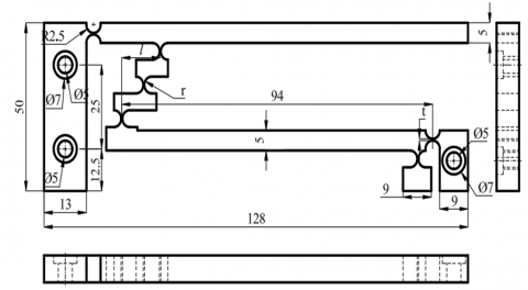
The compliant mechanism amplifier, incorporating a circular elastic joint, has been integrated into Gas–Liquid Thermoelectric Power Equipment, as illustrated in Figure 1. The overall dimensions of the model measure 128 mm in length, 50 mm in width, and 8 mm in thickness. Figure 2 provides detailed information on the design dimensions and variables used in the model.
Figure 1. Compliant mechanism amplifier model
Figure 2. Projection and dimensions of the amplifier mechanism
The design and evaluation process involved the following steps:
The mechanism was constructed using Autodesk Inventor software to ensure precision in replicating the intended geometry.
A Taguchi design of experiments was employed to systematically define the variations of design parameters. Based on this, 27 models were generated for analysis.
Material type, represented by Poisson’s ratio (p), included three materials:
Magnesium alloy (p = 0.29)
Titanium alloy (p = 0.31)
Aluminum alloy (p = 0.33)
Bending hinge thickness (t) was tested at three levels: 0.25 mm, 0.30 mm, and 0.35 mm.
The distance between the two bending hinges (l) was varied at 10 mm, 12 mm, and 14 mm.
Radius of the circular bending hinge (r) was set at 2.0 mm, 2.5 mm, and 3.0 mm.
Each of the 27 model variations combined different levels of these four parameters to cover the full factorial design space.
2.2 Analysis of the elastic displacement amplifier
To analyze the stress and displacement of the compliant mechanism amplifier using the static analysis module of ANSYS software, the following steps are performed:
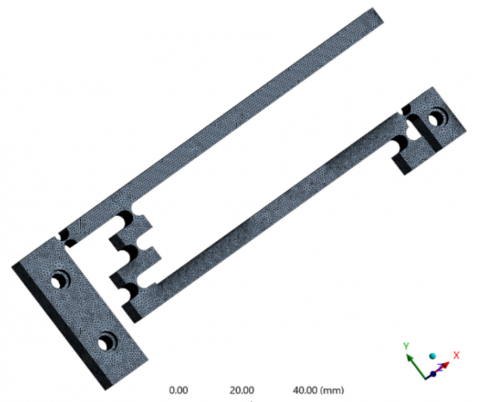
Figure 3. Finite element model
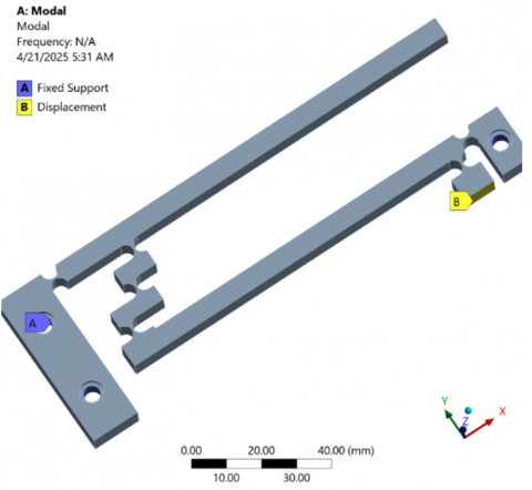
Figure 4. Input load and boundary condition setup
3.1 Determine the weight
The weight of each objective was determined using the MEREC method [24-28] as follows:
Step 1: Build an m×n matrix where each element xij>0 represents the performance of alternative i under criterion j.
Step 2: Normalize the Decision Matrix:
Apply linear normalization to scale values, treating beneficial and cost criteria differently:
$h_{i j}=\frac{\min u_{i j}}{u_{i j}}$ For beneficial criteria (1)
$h_{i j}=\frac{u_{i j}}{\max u_{i j}}$ For bad criteria (2)
uij are the stress and displacement values estimated by FEM.
Step 3: Determine performance for each case:
$S_i=\ln \left[1+\left(\frac{1}{n} \sum_j^n\left|\ln \left(h_{i j}\right)\right|\right)\right]$ (3)
Step 4: Determine effective performance after eliminating individual criteria:
$S_{i j}^{\prime}=\ln \left[1+\left(\frac{1}{n} \sum_{k, k \neq j}^n\left|\ln \left(h_{i j}\right)\right|\right)\right]$ (4)
Step 5: Determine the standard deviation:
$E_j=\left|S_{i j}^{\prime}-S_i\right|$ (5)
Step 6: Derive final criteria weights:
Normalize the removal effects to obtain weights:
$w_j=\frac{E_j}{\sum_k^m E_k}$ (6)
3.2 SAW method
Step 1: Determine the standardized value of each criterion [29-32] as follows:
Step 2: Determine the standardized value of each criterion:
$n_{i j}=\frac{y_{i j}}{\max y_{i j}}$ For beneficial criteria (7)
$n_{i j}=\frac{\min y_{i j}}{y_{i j}}$ For bad criteria (8)
Step 3: Determine the weight normalization value:
$v_i=\sum_{j=1}^n w_j . n_{i j}$ (9)
where, wj is the weight of each objective, determined by the MEREC method.
Step 4: Determine the rank of vi
The optimal case is the case with the largest value of vi.
4.1 Simulation setup
In this investigation, displacement and stress in the compliant mechanism amplifier were analyzed using four design parameters, as outlined in Table 1:
Table 1. Design parameters
|
Designed Dimension |
Symbol |
Unit |
Level 1 |
Level 2 |
Level 3 |
|
Poisson ratio |
p |
mm |
0.29 |
0.31 |
0.33 |
|
Thickness of flexure hinge |
t |
mm |
0.25 |
0.3 |
0.35 |
|
Distance between two flexure hinges |
l |
mm |
10 |
12 |
14 |
|
Radius of circular flexure hinge |
r |
mm |
2.5 |
3.0 |
3.5 |
The results of finite element analyses across all 27 parameter combinations are recorded in Table 2. The variation in displacement and stress among these cases clearly demonstrates that changes in design dimensions significantly affect the mechanism’s performance.
Table 2. Orthogonal array and finite element analysis results
|
Order |
p |
t |
l |
r |
Displacement (mm) |
Stress (MPa) |
|
1 |
0.29 |
0.25 |
10.00 |
2.00 |
0.42012 |
95.662 |
|
2 |
0.29 |
0.25 |
12.00 |
2.50 |
0.59364 |
74.308 |
|
3 |
0.29 |
0.25 |
14.00 |
3.00 |
0.59016 |
82.376 |
|
4 |
0.29 |
0.30 |
10.00 |
2.50 |
0.57782 |
69.948 |
|
5 |
0.29 |
0.30 |
12.00 |
3.00 |
0.58155 |
73.483 |
|
6 |
0.29 |
0.30 |
14.00 |
2.00 |
0.67342 |
60.137 |
|
7 |
0.29 |
0.35 |
10.00 |
3.00 |
0.56912 |
69.954 |
|
8 |
0.29 |
0.35 |
12.00 |
2.00 |
0.58155 |
73.479 |
|
9 |
0.29 |
0.35 |
14.00 |
2.50 |
0.59424 |
69.681 |
|
10 |
0.31 |
0.25 |
10.00 |
2.00 |
0.53309 |
69.893 |
|
11 |
0.31 |
0.25 |
12.00 |
2.50 |
0.56147 |
69.694 |
|
12 |
0.31 |
0.25 |
14.00 |
3.00 |
0.49346 |
58.775 |
|
13 |
0.31 |
0.30 |
10.00 |
2.50 |
0.53309 |
69.893 |
|
14 |
0.31 |
0.30 |
12.00 |
3.00 |
0.50272 |
60.163 |
|
15 |
0.31 |
0.30 |
14.00 |
2.00 |
0.50243 |
59.312 |
|
16 |
0.31 |
0.35 |
10.00 |
3.00 |
0.49663 |
61.657 |
|
17 |
0.31 |
0.35 |
12.00 |
2.00 |
0.5648 |
58.956 |
|
18 |
0.31 |
0.35 |
14.00 |
2.50 |
0.44536 |
58.182 |
|
19 |
0.33 |
0.25 |
10.00 |
2.00 |
0.43914 |
60.451 |
|
20 |
0.33 |
0.25 |
12.00 |
2.50 |
0.43802 |
58.012 |
|
21 |
0.33 |
0.25 |
14.00 |
3.00 |
0.44794 |
58.26 |
|
22 |
0.33 |
0.30 |
10.00 |
2.50 |
0.5468 |
60.489 |
|
23 |
0.33 |
0.30 |
12.00 |
3.00 |
0.4546 |
62.792 |
|
24 |
0.33 |
0.30 |
14.00 |
2.00 |
0.43217 |
58.726 |
|
25 |
0.33 |
0.35 |
10.00 |
3.00 |
0.45005 |
62.898 |
|
26 |
0.33 |
0.35 |
12.00 |
2.00 |
0.35379 |
54.57 |
|
27 |
0.33 |
0.35 |
14.00 |
2.50 |
0.43293 |
57.164 |
4.2 Weighting results
The weights are determined using the MEREC method, and the results are recorded by inputting the displacement (Di) and stress (St) values into Eqs. (1) and (2), as shown in Table 3. The second and third columns display the results of Eq. (1) and (2), respectively. The fourth column presents the outcome of Eq. (3). The fifth and sixth columns show the results of Eq. (4). The seventh and eighth columns contain the results of Eq. (5). The weights for displacement and stress are calculated as 0.714 and 0.286, respectively, according to Eq. (6).
Table 3. Weight determination results
|
TT |
hij |
Si |
Sij' |
Ej |
|||
|
Di |
St |
Di |
St |
Di |
St |
||
|
1 |
0.6239 |
1.0000 |
0.2118 |
0.2118 |
0.0000 |
0.0000 |
0.2118 |
|
2 |
0.8815 |
0.7768 |
0.1734 |
0.0611 |
0.1189 |
0.1123 |
0.0578 |
|
3 |
0.8764 |
0.8611 |
0.1317 |
0.0639 |
0.0721 |
0.0678 |
0.0082 |
|
4 |
0.8580 |
0.7312 |
0.2095 |
0.0738 |
0.1454 |
0.1358 |
0.0717 |
|
5 |
0.8636 |
0.7682 |
0.1867 |
0.0708 |
0.1239 |
0.1159 |
0.0531 |
|
6 |
1.0000 |
0.6286 |
0.2087 |
0.0000 |
0.2087 |
0.2087 |
0.2087 |
|
7 |
0.8451 |
0.7313 |
0.2156 |
0.0808 |
0.1454 |
0.1348 |
0.0646 |
|
8 |
0.8636 |
0.7681 |
0.1867 |
0.0708 |
0.1239 |
0.1159 |
0.0531 |
|
9 |
0.8824 |
0.7284 |
0.1997 |
0.0607 |
0.1471 |
0.1390 |
0.0864 |
|
10 |
0.7916 |
0.7306 |
0.2420 |
0.1105 |
0.1458 |
0.1315 |
0.0353 |
|
11 |
0.8338 |
0.7285 |
0.2226 |
0.0870 |
0.1470 |
0.1355 |
0.0600 |
|
12 |
0.7328 |
0.6144 |
0.3358 |
0.1445 |
0.2180 |
0.1913 |
0.0735 |
|
13 |
0.7916 |
0.7306 |
0.2420 |
0.1105 |
0.1458 |
0.1315 |
0.0353 |
|
14 |
0.7465 |
0.6289 |
0.3207 |
0.1364 |
0.2085 |
0.1842 |
0.0721 |
|
15 |
0.7461 |
0.6200 |
0.3260 |
0.1367 |
0.2143 |
0.1894 |
0.0776 |
|
16 |
0.7375 |
0.6445 |
0.3162 |
0.1417 |
0.1985 |
0.1745 |
0.0568 |
|
17 |
0.8387 |
0.6163 |
0.2852 |
0.0843 |
0.2167 |
0.2009 |
0.1324 |
|
18 |
0.6613 |
0.6082 |
0.3753 |
0.1879 |
0.2220 |
0.1873 |
0.0341 |
|
19 |
0.6521 |
0.6319 |
0.3669 |
0.1937 |
0.2066 |
0.1732 |
0.0129 |
|
20 |
0.6504 |
0.6064 |
0.3819 |
0.1948 |
0.2232 |
0.1872 |
0.0284 |
|
21 |
0.6652 |
0.6090 |
0.3728 |
0.1855 |
0.2215 |
0.1873 |
0.0360 |
|
22 |
0.8120 |
0.6323 |
0.2877 |
0.0991 |
0.2063 |
0.1886 |
0.1073 |
|
23 |
0.6751 |
0.6564 |
0.3414 |
0.1794 |
0.1910 |
0.1621 |
0.0117 |
|
24 |
0.6418 |
0.6139 |
0.3824 |
0.2003 |
0.2183 |
0.1821 |
0.0180 |
|
25 |
0.6683 |
0.6575 |
0.3444 |
0.1836 |
0.1903 |
0.1608 |
0.0068 |
|
26 |
0.5254 |
0.5704 |
0.4716 |
0.2790 |
0.2474 |
0.1925 |
0.0316 |
|
27 |
0.6429 |
0.5976 |
0.3909 |
0.1996 |
0.2291 |
0.1913 |
0.0295 |
4.3 SAW method optimization results
The results obtained from the SAW method are recorded by inputting the displacement (Di) and stress (St) values into Eq. (7) and Eq. (8), as detailed in Table 4. The second and third columns of the table present the outcomes of these equations, respectively. The fourth column displays the result derived from Eq. (9), while the fifth column ranks the Vi values. The model with the highest Vi value is ranked first, continuing sequentially until the model with the lowest Vi value was ranked 27th. As indicated in the table, the sixth model, which holds the highest Vi value, was identified as the optimal case. This optimal model comprises the following specifications: a material Poisson's ratio of 0.29, a circular hinge thickness of 0.3 mm, a distance between two circular elastic joints (l) of 14 mm, and a radius of the circular elastic joint (r) of 2 mm. The corresponding optimal Vi value is 0.97353, with an optimal displacement of 0.67342 mm and an optimal stress of 60.137 MPa. The distinct Vi values across the models underscore the significant impact of the design dimensions on the displacement and stress characteristics of the amplifier compliance mechanism with a bending hinge. These findings align with the results obtained from finite element analysis.
Table 4. Results of SAW method
|
Order |
nij |
Vi |
Rank |
|
|
Di |
St |
|||
|
1 |
0.62386 |
0.57045 |
0.60858 |
27 |
|
2 |
0.88153 |
0.73438 |
0.83945 |
4 |
|
3 |
0.87636 |
0.66245 |
0.81519 |
11 |
|
4 |
0.85804 |
0.78015 |
0.83576 |
6 |
|
5 |
0.86358 |
0.74262 |
0.82899 |
8 |
|
6 |
1.00000 |
0.90743 |
0.97353 |
1 |
|
7 |
0.84512 |
0.78008 |
0.82652 |
9 |
|
8 |
0.86358 |
0.74266 |
0.82900 |
7 |
|
9 |
0.88242 |
0.78314 |
0.85403 |
3 |
|
10 |
0.79162 |
0.78076 |
0.78851 |
15 |
|
11 |
0.83376 |
0.78299 |
0.81924 |
10 |
|
12 |
0.73277 |
0.92846 |
0.78873 |
14 |
|
13 |
0.79162 |
0.78076 |
0.78851 |
15 |
|
14 |
0.74652 |
0.90704 |
0.79242 |
13 |
|
15 |
0.74609 |
0.92005 |
0.79584 |
12 |
|
16 |
0.73747 |
0.88506 |
0.77968 |
17 |
|
17 |
0.83870 |
0.92561 |
0.86356 |
2 |
|
18 |
0.66134 |
0.93792 |
0.74044 |
19 |
|
19 |
0.65210 |
0.90271 |
0.72377 |
25 |
|
20 |
0.65044 |
0.94067 |
0.73344 |
20 |
|
21 |
0.66517 |
0.93666 |
0.74281 |
18 |
|
22 |
0.81197 |
0.90215 |
0.83776 |
5 |
|
23 |
0.67506 |
0.86906 |
0.73054 |
22 |
|
24 |
0.64175 |
0.92923 |
0.72397 |
24 |
|
25 |
0.66831 |
0.86760 |
0.72530 |
23 |
|
26 |
0.52536 |
1.00000 |
0.66110 |
26 |
|
27 |
0.64288 |
0.95462 |
0.73203 |
21 |
4.4 Confirmation of results by Taguchi method
The results of the Taguchi analysis (signal-to-noise analysis) confirmed that the design parameters significantly influenced the displacement and stress of the elastic amplifier mechanism. This is evident from the largest deviations in the signal-to-noise ratios of the variables across different levels. As shown in Table 5, the deviation values of the signal-to-noise ratios for the design parameters are as follows:
Accordingly, variable p has the greatest influence, followed by variable t, variable r, and finally variable l.
Table 5. Signal/noise analysis results
|
Level |
p |
t |
l |
r |
|
1 |
-1.743 |
-2.394 |
-2.301 |
-2.328 |
|
2 |
-1.997 |
-1.840 |
-1.977 |
-2.091 |
|
3 |
-2.694 |
-2.199 |
-2.156 |
-2.015 |
|
Delta |
0.952 |
0.554 |
0.323 |
0.313 |
|
Rank |
1 |
2 |
3 |
4 |
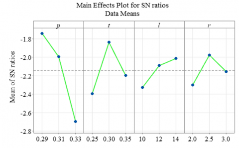
Figure 5. Signal/noise analysis graph
The data presented in Table 5 were utilized to construct a signal-to-noise ratio (S/N) graph, as shown in Figure 5. This graph clearly indicates that the optimal configuration corresponds to the highest peak, confirming the findings. Specifically, the optimal case is the sixth model, which features a magnesium alloy material, a circular elastic joint thickness of 0.30 mm, a distance between the two circular elastic joints (l) of 14.00 mm, and a circular elastic joint radius (r) of 2.00 mm. The resulting optimal displacement and stress values are 0.67342 mm and 60.137 MPa, respectively.
The graph further illustrates that the design parameters significantly influence the displacement and stress. The steepness of the graph's slope correlates with the extent of each parameter's impact. Notably, the material exhibits the greatest influence, as indicated by the steepest slope, followed by the thickness (t), distance (l), and radius (r) variables.
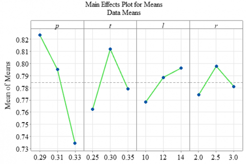
Similarly to the signal-to-noise analysis results, the mean value analysis also confirms that the design parameters significantly affect the displacement and stress of the elastic displacement amplifier, as indicated by the deflection values. Larger deflections correspond to greater impacts on displacement and stress. Specifically, the material's Poisson's ratio has the most substantial effect, followed by the thickness (t) of the circular elastic joint, the distance (l) between the two elastic joints, and finally the radius (r) of the circular elastic joint. The respective deflection values for the variables p, t, l, and r are 0.0889, 0.0497, 0.0280, and 0.0236.
Table 6. Average value analysis results
|
Level |
p |
t |
l |
r |
|
1 |
0.8234 |
0.7622 |
0.7683 |
0.7742 |
|
2 |
0.7952 |
0.8119 |
0.7886 |
0.7979 |
|
3 |
0.7345 |
0.7791 |
0.7963 |
0.7811 |
|
Delta |
0.0889 |
0.0497 |
0.0280 |
0.0236 |
|
Rank |
1 |
2 |
3 |
4 |
Similarly, the data presented in Table 6 were utilized to construct an average value plot. This graph clearly indicates that the optimal case corresponds to the highest peak, confirming the findings. Specifically, the optimal model was the sixth model, which features a magnesium alloy material, a circular elastic joint thickness of 0.30 mm, a distance between the two circular elastic joints (l) of 14.00 mm, and a circular elastic joint radius (r) of 2.00 mm. The resulting optimal displacement and stress values are 0.67342 mm and 60.137 MPa, respectively.
Figure 6 further illustrates that the design parameters significantly influence the displacement and stress. The steepness of the graph's slope correlates with the extent of each parameter's impact. Notably, the material exhibits the greatest influence, as indicated by the steepest slope, followed by the thickness (t), distance (l), and radius (r) variables.
Figure 6. Average value analysis graph
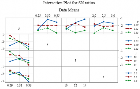
To validate the results obtained from the finite element analysis and the SAW method, an interaction analysis of the signal-to-noise ratios was conducted, as shown in Figure 7. The interaction plot reveals non-parallel lines, signifying that the design parameters have a substantial effect on the displacement and stress of the elastic displacement amplifier mechanism.
Figure 7. Signal/noise interaction analysis graph
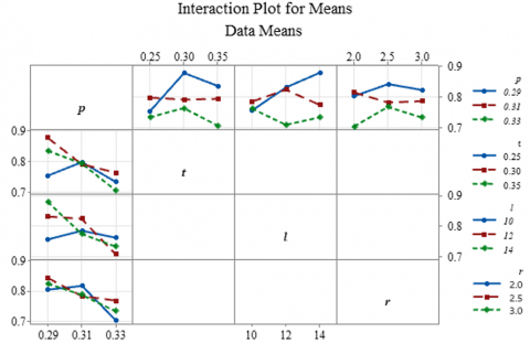
Additionally, to further confirm the findings, an interaction analysis of the mean values was performed and is presented in Figure 8. Similar to the previous analysis, the interaction plot demonstrates non-parallel lines, reinforcing the conclusion that the design parameters significantly affect the displacement and stress of the elastic displacement amplifier.
Figure 8. Average value interaction analysis graph
The ANOVA results as illustrated in Table 7 indicated that the regression model is statistically significant, as shown by the overall F-value of 806.00 and a p-value of 0.000. The model accounts for 99.46% of the total variation in the response variable, reflecting an excellent fit. Among the predictors, variable p stands out with the largest contribution (98.45%) and a highly significant p-value, indicating it plays a major role in explaining the outcome. The quadratic term pp is also statistically significant, suggesting a nonlinear effect of p. Variables t and l show moderate contributions and are significant at the 5% level. However, variable r has a weaker impact and is only marginally significant, with a p-value of 0.082. The very low error variance further confirms the model’s strong performance and reliability.
Table 7. Analysis of variance
|
Source |
DF |
Seq SS |
Contribution |
Adj SS |
Seq MS |
F-Value |
P-Value |
|
Regression |
5 |
16.6540 |
99.46% |
16.6540 |
3.3308 |
806.00 |
0.000 |
|
p |
1 |
16.4858 |
98.45% |
0.1020 |
16.4858 |
3989.30 |
0.000 |
|
t |
1 |
0.0319 |
0.19% |
0.0013 |
0.0319 |
7.72 |
0.011 |
|
l |
1 |
0.0320 |
0.19% |
0.0035 |
0.0320 |
7.75 |
0.011 |
|
r |
1 |
0.0137 |
0.08% |
0.0002 |
0.0137 |
3.32 |
0.082 |
|
p*p |
1 |
0.0905 |
0.54% |
0.0905 |
0.0905 |
21.90 |
0.000 |
|
Error |
22 |
0.0909 |
0.54% |
0.0909 |
0.0041 |
|
|
|
Total |
27 |
16.7449 |
100.00% |
|
|
|
|
The summary statistics as recorded in Table 8 indicate that the regression model provides an excellent fit to the data. The R-squared value of 99.46% suggests that the model explains nearly all of the variability in the response variable. The adjusted R-squared is also high at 99.33%, confirming that the model remains robust even after accounting for the number of predictors. The predicted R-squared value of 99.13% demonstrates strong predictive accuracy on unseen data. Additionally, the small standard error (S = 0.0643) and low PRESS value (0.1462) further support the model’s reliability. The negative AICc and BIC values indicate a well-optimized model with both strong explanatory power and minimal complexity.
Table 8. Model summary
|
S |
R-sq |
R-sq (adj) |
PRESS |
R-sq (pred) |
AICc |
BIC |
|
0.0642846 |
99.46% |
99.33% |
0.146206 |
99.13% |
-60.91 |
-57.33 |
Regression Equation
Vi = - 13.81 p2 +6.33 p + 0.167 t + 0.00696 l + 0.0067 r
The results of the analysis of variance yielded the regression equation as presented in Eq. (10). The regression equation shows how the response variable Vi was influenced by several predictors. The presence of the squared term p2 with a negative coefficient (-13.81) alongside a positive linear term for p (6.33) indicated a nonlinear relationship between p and Vi, likely forming a parabolic curve that opens downward. This suggested that Vi increased with variable (p) up to a certain point, then begins to decrease as (p) continued to rise. The coefficients for the other variables (t), (l), and (r) are all positive but relatively small, implying they have a more modest effect on Vi. Overall, the model captures both linear and nonlinear influences, with (p) being the most impactful predictor due to its strong linear and quadratic terms.
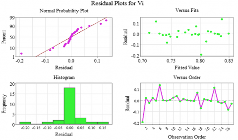
The residual plots as depicted in Figure 9 suggested that the regression model satisfies the main assumptions. The normal probability plot shows that the residuals follow a roughly straight line, indicating they are approximately normally distributed. The histogram supports this by displaying a fairly symmetric shape centered around zero. In the plot of residuals versus fitted values, the points are randomly scattered without any clear pattern, suggesting constant variance. Additionally, the plot of residuals versus observation order shows no noticeable trends or cycles, which implies that there is no autocorrelation. Overall, these diagnostic plots confirm that the model is statistically reliable and well-fitted.
Figure 9. Residual plots
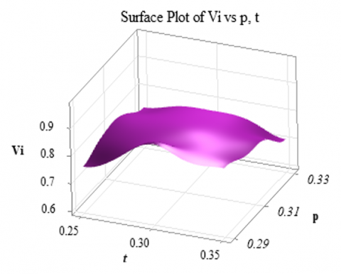
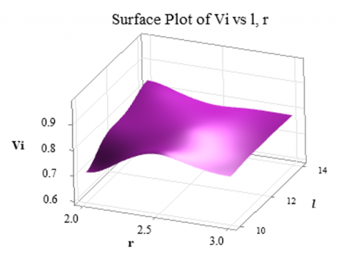
To further validate the results obtained from the finite element analysis, SAW method, and Taguchi method, a 3D surface graph analysis was conducted, as shown in Figure 10 and Figure 11. The graph revealed several key trends:
These observations underscore the significant influence of design parameters on the displacement and stress characteristics of the elastic displacement amplifier mechanism.
Figure 10. Relationship between Vi and p and t
Figure 11. The relationship between Vi and l and r
The comparison between finite element simulation results and Taguchi method predictions is detailed in Table 9. This table demonstrates that the discrepancies between the simulated and predicted values remain within 3%, indicating a high degree of agreement between the two approaches. Such small deviations well within acceptable scientific thresholds underscore the reliability of the predictive method.
Table 9. Comparison of predicted values and finite element analysis values
|
Di FEM |
Di Predicted |
Error (%) |
St FEM |
St Predicted |
Error (%) |
Vi FEM |
Vi Predicted |
Eror |
|
0.4201 |
0.4289 |
2.04 |
95.662 |
94.3898 |
1.35 |
0.60858 |
0.618168 |
1.55 |
|
0.5936 |
0.5873 |
1.08 |
74.308 |
75.5114 |
1.59 |
0.83945 |
0.830651 |
1.06 |
|
0.5902 |
0.5827 |
1.28 |
82.376 |
81.4448 |
1.14 |
0.81519 |
0.811987 |
0.39 |
|
0.5778 |
0.5704 |
1.30 |
69.948 |
69.0168 |
1.35 |
0.83576 |
0.832563 |
0.38 |
|
0.5816 |
0.5953 |
2.31 |
73.483 |
72.2108 |
1.76 |
0.82899 |
0.838569 |
1.14 |
|
0.6734 |
0.6710 |
0.37 |
60.137 |
60.3404 |
0.34 |
0.97353 |
0.977144 |
0.37 |
|
0.5691 |
0.5728 |
0.64 |
69.954 |
70.1574 |
0.29 |
0.82652 |
0.800138 |
3.30 |
|
0.5816 |
0.5741 |
1.30 |
73.479 |
72.5478 |
1.28 |
0.82900 |
0.825797 |
0.39 |
|
0.5942 |
0.6080 |
2.26 |
69.681 |
69.0878 |
0.86 |
0.85403 |
0.843612 |
1.23 |
|
0.5331 |
0.5442 |
2.03 |
69.893 |
70.9422 |
1.48 |
0.78851 |
0.809937 |
2.65 |
|
0.5615 |
0.5561 |
0.97 |
69.694 |
70.8689 |
1.66 |
0.81924 |
0.816203 |
0.37 |
|
0.4935 |
0.4878 |
1.16 |
58.775 |
59.1809 |
0.69 |
0.78873 |
0.770345 |
2.39 |
|
0.5331 |
0.5274 |
1.07 |
69.893 |
70.2989 |
0.58 |
0.78851 |
0.770127 |
2.39 |
|
0.5027 |
0.5138 |
2.15 |
60.163 |
60.3642 |
0.33 |
0.79242 |
0.813846 |
2.63 |
|
0.5024 |
0.4970 |
1.09 |
59.312 |
58.7049 |
1.03 |
0.79584 |
0.792798 |
0.38 |
|
0.4966 |
0.4912 |
1.10 |
61.657 |
61.0499 |
0.99 |
0.77968 |
0.776642 |
0.39 |
|
0.5648 |
0.5491 |
2.85 |
58.956 |
59.3619 |
0.68 |
0.86356 |
0.845171 |
2.18 |
|
0.4454 |
0.4564 |
2.42 |
58.182 |
58.3832 |
0.34 |
0.74044 |
0.76186 |
2.81 |
|
0.4391 |
0.4409 |
0.39 |
60.451 |
59.5778 |
1.47 |
0.72377 |
0.729516 |
0.79 |
|
0.438 |
0.4419 |
0.87 |
58.012 |
57.3958 |
1.07 |
0.73344 |
0.740397 |
0.94 |
|
0.4479 |
0.4424 |
1.26 |
58.26 |
59.7494 |
2.49 |
0.74281 |
0.730113 |
1.74 |
|
0.5468 |
0.5412 |
1.03 |
60.489 |
61.9784 |
2.40 |
0.83776 |
0.825063 |
1.54 |
|
0.4546 |
0.4563 |
0.38 |
62.792 |
61.9188 |
1.41 |
0.73054 |
0.736283 |
0.78 |
|
0.4322 |
0.4360 |
0.88 |
58.726 |
58.1098 |
1.06 |
0.72397 |
0.730923 |
0.95 |
|
0.4501 |
0.4539 |
0.85 |
62.898 |
62.2818 |
0.99 |
0.72530 |
0.732255 |
0.95 |
|
0.3538 |
0.3482 |
1.60 |
54.57 |
56.0594 |
2.66 |
0.66110 |
0.6484 |
1.96 |
|
0.4329 |
0.4346 |
0.39 |
57.164 |
56.2908 |
1.55 |
0.73203 |
0.737776 |
0.78 |
Table 10. Compare the predicted value and the optimal value
|
Di Optimal |
Di Predicted |
Error (%) |
St Optimal |
St Predicted |
Error (%) |
Vi Optimal |
Vi Predicted |
Eror (%) |
|
0.6734 |
0.6710 |
0.37 |
60.137 |
60.3404 |
0.34 |
0.97353 |
0.977144 |
0.37 |
The reliability of the SAW method was confirmed by comparing its optimal results with those predicted by the Taguchi approach, as recorded in Table 10. The discrepancies in Di, St, and Vi were minima, only 0.37%, 0.34%, and 0.37%, respectively, well under the 1% threshold, affirming the method’s accuracy.
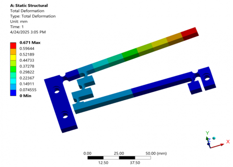
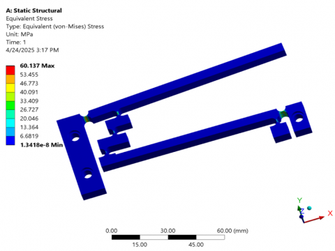
The optimum results of displacement and stress were obtained as 0.671 mm and 60.137 MPa, as shown in Figure 12 and Figure 13, respectively.
Figure 12. Optimal displacement
Figure 13. Optimal stress
This investigation evaluated 27 elastic displacement amplifier models via finite element analysis. Key findings:
The investigation assumed linear elastic behavior, omits experimental validation, and ignores dynamic, thermal, or multi-physics effects.
Future work:
Apply advanced optimization (e.g., response surface methodology, genetic algorithms, machine learning) for multi-objective design.
This work was partially financially supported by Ho Chi Minh City University of Industry and Trade under Contract No. 28/HĐ-DCT, dated on January 17, 2025.
[1] Huang, L., Shen, Z.J. (2022). Design and optimization of amplifying mechanism in gas-liquid thermoelectric power device. Journal of Physics: Conference Series, 2355(1): 1-7. https://iopscience.iop.org/article/10.1088/1742-6596/2355/1/012033
[2] Zhang, W., Yan, P. (2024). A variable stiffness compliant actuator based on antagonistic normal-stressed electromagnetic mechanism. Sensors and Actuators A: Physical, 366: 1-14. https://doi.org/10.1016/j.sna.2023.114983
[3] Paniselvam, V., Tan, N.Y.J., Anantharajan, S.K. (2023). A review on the design and application of compliant mechanism-based fast-tool servos for ultraprecision machining. Machines, 11(4): 1-36. https://doi.org/10.3390/machines11040450
[4] Meyer, P., Finder, J., Hühne, C. (2023). Test methods for the mechanical characterization of flexure hinges. Experimental Mechanics, 63(7): 1203-1222. https://doi.org/10.1007/s11340-023-00982-7
[5] Wang, Y., Zhang, L., Meng, L., Lu, H., Ma, Y. (2024). Theoretical modeling and experimental verification of elliptical hyperbolic hybrid flexure hinges. Symmetry, 16(3): 1-20. https://doi.org/10.3390/sym16030345
[6] Wei, H., Tian, Y., Zhao, Y., Ling, M., Shirinzadeh, B. (2023). Two-axis flexure hinges with variable elliptical transverse cross-sections. Mechanism and Machine Theory, 181: 105183. https://doi.org/10.1016/j.mechmachtheory.2022.105183
[7] Wu, H., Tang, H., Qin, Y. (2024). Design and test of a 2-DOF compliant positioning stage with antagonistic piezoelectric actuation. Machines, 12(6): 1-13. https://doi.org/10.3390/machines12060420
[8] Sun, J., Hu, H. (2024). Dynamic topology optimization of flexible multibody systems. Nonlinear Dynamics, 112(14): 11711-11743. https://doi.org/10.1007/s11071-024-09619-3
[9] Shi, H., Yang, G., Li, H.N., Zhao, J., Yu, H., Zhang, C. (2024). A flexure-based and motion-decoupled XYZ nano-positioning stage with a quasi-symmetric structure. Precision Engineering, 89: 239-251. https://doi.org/10.1016/j.precisioneng.2024.06.014
[10] Das, T.K., Shirinzadeh, B. (2024). Design, computational analysis and experimental study of a high amplification piezoelectric actuated microgripper. Engineering Research Express, 6(3): 1-16. https://doi.org/10.1088/2631-8695/ad5f19
[11] Chen, W., Zhang, Y., Wang, X., Li, J., Liu, H., Zhao, K., Sun, M. (2024). Nonlinear design, analysis, and testing of a single-stage compliant orthogonal displacement amplifier with a single input force for microgrippers. Journal of Micromechanics and Microengineering, 34(7): 1-17. https://iopscience.iop.org/article/10.1088/1361-6439/ad5a19.
[12] Gan, J., Xie, W., Yang, W., Lei, S., Lei, B. (2025). Design of a novel Z-shaped flexure hinge and a 2DOF XY precision positioning platform. Precision Engineering, 93: 459-469. https://doi.org/10.1016/j.precisioneng.2025.01.026
[13] Jani, N., Tirupathi, R., Menon, P.K., Pandey, A.K. (2025). Modelling and optimization of compound lever-based displacement amplifier in a MEMS accelerometer. Microsystem Technologies, 31(6): 1337-1356. https://doi.org/10.1007/s00542-024-05757-1
[14] Zhang, M., Zhao, Q., Li, Z., Wang, S., He, G., Zhao, L. (2025). Development of a piezoelectric resonator with in-plane displacement-amplification mechanism. Microsystem Technologies, 31(1): 231-243. https://doi.org/10.1007/s00542-024-05743-7
[15] Mansour, M.A., Elsayed, M.M., Ali, A.M., Toraya, A., Gaber, N. (2025). Experimental and numerical investigations of microthermal actuator employing the amplification theory for achieving competitive performance. Scientific Reports, 15(1): 27023. https://doi.org/10.1038/s41598-025-11763-8
[16] Liu, M., Wang, J., Chen, X., Zhang, L., Li, Y., Zhao, H., Sun, W. (2025). Design and development of a 3-DOF compliant gripper with in-plane and out-of-plane motion. Precision Engineering, 95: 136-150. https://doi.org/10.1016/j.precisioneng.2025.04.019
[17] Knapkiewicz, P., Kawa, B. (2025). Long travel and high gain, miniature piezo-stack actuator amplifier. Experimental Techniques, 1-13. https://link.springer.com/article/10.1007/s40799-025-00821-5.
[18] Tissot-Daguette, L., Cosandier, F., Gubler, Q., Pétremand, Y., Despont, M., Henein, S. (2025). Residual stress chevron preloading amplifier for large-stroke stiffness reduction of silicon flexure mechanisms. Journal of Micromechanics and Microengineering, 35(2): 025003. https://doi.org/10.1088/1361-6439/ada165
[19] Wang, R., Yang, L., Li, Z., Wang, H., Zhang, X. (2025). Design and control of a piezoelectric-actuated kangaroo-inspired bionic compliant mechanism for LDI machines. Chinese Journal of Mechanical Engineering, 38(1): 1-13. https://doi.org/10.1186/s10033-025-01307-6
[20] Xu, M., Yang, Y., Lv, Y., Wu, G., Cui, Y. (2025). A novel bionic parallel XY piezoelectric stick-slip positioning stage. Precision Engineering, 92: 1-20. https://doi.org/10.1016/j.precisioneng.2024.11.009
[21] Ren, J., Shu, Y., Lin, Y. (2025). Kinetostatic modeling and workspace analysis of redundant actuated n-4R compliant parallel pointing mechanism. Micromachines, 16(6): 1-20. https://doi.org/10.3390/mi16040478
[22] Khaleel, H.H. (2023). Stress analysis of gas turbine propeller using finite elements method. Mathematical Modelling of Engineering Problems, 10(1): 236-241. https://doi.org/10.18280/mmep.100127
[23] Kadhom, H.K., Mohammed, A.J., Sillanpää, M. (2024). The influence of thickness and interference fit ratio on fatigue phenomenon: An empirical study. Mathematical Modelling of Engineering Problems, 11(1): 1-17. https://doi.org/10.18280/mmep.110101
[24] Keshavarz-Ghorabaee, M., Amiri, M., Zavadskas, E.K., Turskis, Z., Antucheviciene, J. (2021). Determination of objective weights using a new method based on the removal effects of criteria (MEREC). Symmetry, 13(4): 525. https://doi.org/10.3390/sym13040525
[25] Keshavarz-Ghorabaee, M. (2021). Assessment of distribution center locations using a multi-expert subjective-objective decision-making approach. Scientific Reports, 11(1): 19461. https://doi.org/10.1038/s41598-021-98698-y
[26] Borchers, A., Pieler, T. (2010). Programming pluripotent precursor cells derived from Xenopus embryos to generate specific tissues and organs. Genes, 1(3): 413-426. https://doi.org/10.3390/genes1030413
[27] Shanmugasundar, G., Sapkota, G., Čep, R., Kalita, K. (2022). Application of MEREC in multi-criteria selection of optimal spray-painting robot. Processes, 10(6): 1172. https://doi.org/10.3390/pr10061172
[28] Fan, J., Lei, T., Wu, M. (2024). MEREC-MABAC method based on cumulative prospect theory for picture fuzzy sets: Applications to wearable health technology devices. Expert Systems with Applications, 255: 1-20. https://doi.org/10.1016/j.eswa.2024.124749
[29] Tafazzoli, M., Hazrati, A., Shrestha, K., Kisi, K. (2024). Enhancing contractor selection through fuzzy TOPSIS and fuzzy SAW techniques. Buildings, 14(6): 1-12. https://doi.org/10.3390/buildings14061861
[30] Jazaudhi’fi, A., Vitianingsih, A.V., Kristyawan, Y., Maukar, A.L., Yasin, V. (2024). Recommendation system to determine achievement students using Naïve Bayes and simple additive weighting (SAW) methods. Digital Zone: Jurnal Teknologi Informasi dan Komunikasi, 15(1): 67-79. https://doi.org/10.31849/digitalzone.v15i1.19746
[31] Taherdoost, H. (2023). Analysis of simple additive weighting method (SAW) as a multi-attribute decision-making technique: A step-by-step guide. Journal of Management Science and Engineering Research, 6(1): 21-24. https://doi.org/10.30564/jmser.v6i1.5400
[32] Ciardiello, F., Genovese, A. (2023). A comparison between TOPSIS and SAW methods. Annals of Operations Research, 325(2): 967-994. https://doi.org/10.1007/s10479-023-05339-w