Nicco Plamonia*![]() | Ahmad Pratama Putra
| Ahmad Pratama Putra![]() | Ahmad Fauzi Yunus
| Ahmad Fauzi Yunus![]() | Dina Saptiarini
| Dina Saptiarini![]() | Sandy Lesmana
| Sandy Lesmana![]() | Dinda Lutfia Bukit
| Dinda Lutfia Bukit![]() | Sri Wijayanti
| Sri Wijayanti![]() | Dwi Nuraeni A
| Dwi Nuraeni A![]() | Ira Widyastuti
| Ira Widyastuti![]()
© 2025 The authors. This article is published by IIETA and is licensed under the CC BY 4.0 license (http://creativecommons.org/licenses/by/4.0/).
OPEN ACCESS
This study compares the Multi-Utility Tunnel (MUT) method with the conventional method for infrastructure development in the New Capital (IKN), Nusantara, Indonesia, focusing on cost efficiency, soil stability, and sustainability. While the MUT method has a higher initial capital expenditure (IDR 13.25 billion vs. IDR 8.75 billion), it offers significant operational savings, with annual maintenance costs 45% lower than the conventional method. Over 10 years, the total effective cost for MUT is IDR 12.78 billion, compared to IDR 14.25 billion for the conventional method. Soil stability analysis shows that denser soils, particularly in South KIPP (Zone 3), support the MUT system better, reducing soil failure risks. Additionally, the MUT system has slower depreciation (1.25% annually) compared to the conventional method (5%), resulting in a positive asset value after 30 years (IDR 8.28 billion vs. IDR 4.38 billion). This slower depreciation contributes to long-term sustainability by reducing the need for costly repairs. Despite higher initial costs, the MUT method is more cost-effective, stable, and sustainable for large-scale infrastructure projects, offering better long-term returns and operational efficiency.
IKN Nusantara, utility management system, Multi-Utility Tunnel (MUT), sustainability
The Multi-Utility Tunnel (MUT) designed to integrate various utilities within a single tunnel network. The implementation of MUT provides benefits such as integrated utility networks, improved efficiency, longer infrastructure lifespan, support for urban sustainability, easier maintenance, and enhanced safety by reducing physical disruptions [1]. Moreover, MUT systems can be easily integrated with modern innovations and technologies [1, 2], in contrast with traditional utility system places each utility separately, often lacking coordination and neglecting the integration of modern technologies [3, 4]. Traditional systems create several issues, including: (1) high space demand, (2) high operational and maintenance costs, (3) disorganized network management, (4) environmental disturbances from frequent digging, (5) low disaster resilience, (6) low energy efficiency, (7) challenges in integrating new technologies, and (8) negative impacts on the urban economy [5]. Currently, no major city in Indonesia has widely adopted the MUT system. However, the upcoming Nusantara Capital City (IKN), slated for habitation by 2028, offers a unique opportunity to design modern infrastructure, including the MUT. With largely undeveloped land, implementing MUT in IKN is expected to improve sustainable urban functions, optimize space utilization, and provide long-term infrastructure solutions.
This research aims to compare the MUT method and conventional method in terms of sustainability and cost efficiency, focusing on the Core Government Area (KIPP) of IKN Nusantara. It examines long-term sustainability and cost efficiency, using geotechnical data from five KIPP zones, which may not fully represent IKN. The study relies on technical parameters such as cost, soil, and structure, with analysis based on model simulations and real-time tests. Cost estimates are projected over 10 years, excluding contingency and construction-related risks.
This section outlines the research methodology in three sub-sections: (1) Study Location, (2) Data Collection, and (3) Data Analysis Procedure.
2.1 Study location
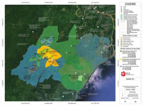
The IKN region spans two regencies, offering a diverse landscape for evaluating infrastructure systems [6, 7]. It covers Penajam Paser Utara Regency (including Penajam and Sepaku sub-districts) and Kutai Kertanegara Regency (comprising Loa Kulu, Loa Janan, Muara Jawa, and Samboja sub-districts). Located between Balikpapan and Samarinda, the IKN region spans 256,142 hectares of land and 68,189 hectares of marine area. The development of IKN is divided into three main zones: (1) Core Government Area (KIPP) – 6,671 hectares, (2) IKN Area (KIKN) – 56,180 hectares, and (3) IKN Development Area (KP IKN) – 199,962 hectares.
The study focuses on the Core Government Area of IKN Nusantara, where the comparison between the MUT method and conventional methods is conducted. The topography of IKN features varying elevations, river basins, and dense forests, presenting significant engineering challenges for infrastructure development (see Figure 1).
Figure 1. Map of study location
2.2 Collection of primary and secondary data
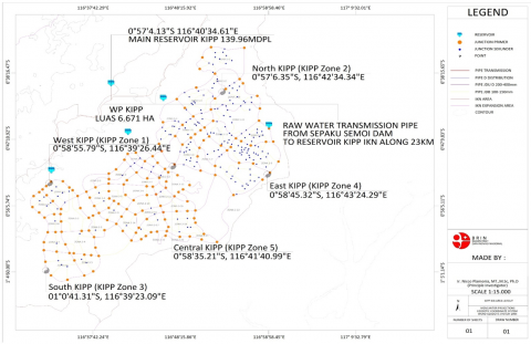
Data for this study were collected over six months, from 11th February 2023 to 23th February 2024, involving stakeholders such as infrastructure developers and relevant institutions responsible for land management and construction. The data was gathered from five locations within the KIPP IKN Zone, which is divided into five zones: Zone 1 (West KIPP Zone), Zone 2 (North KIPP Zone), Zone 3 (South KIPP Zone), Zone 4 (East KIPP Zone), and Zone 5 (Central KIPP Zone) (see Figure 2).
Figure 2. Map of study location
2.2.1 Collection of primary data
Various field surveys must be conducted to gather both spatial and non-spatial data, which collectively information, see Table 1.
Table 1. Primary data collection
|
No. |
Type of Data |
Survey Name |
Data Collected |
Units |
Notes |
|
1 |
Surface elevation and terrain features |
Topographic Survey |
Ground elevation, contour lines, building positions |
meters, UTM |
Required for MUT alignment and cross-section planning |
|
2 |
Precise geolocation of survey points |
Total Station / GNSS |
X, Y, Z coordinates of key points |
meters, decimal degrees |
Georeferenced base map |
|
3 |
Current drainage system conditions |
Drainage Survey |
Drainage dimensions, flow direction, flood-prone points |
m, m², m³/s |
For integrating water channels into MUT |
|
4 |
Underground utility mapping |
Utility Mapping Survey |
Utility types, positions, depth, dimensions |
meters, mm |
Uses trenching or electromagnetic locator tools |
|
5 |
Utility space and layout requirements |
Utility Demand Assessment |
Pipe/cable diameters, required space |
mm, m², m³ |
Determines MUT compartment sizing and configuration |
Soil measurements were conducted at five locations through a Geotechnical Survey to evaluate characteristics impacting MUT design and sustainability. Key data collected, such as soil type, SPT N-value, cohesion, friction angle, groundwater depth, and bearing capacity, are essential for determining tunnel depth and structural lining (see Table 1). These measurements are crucial due to varying soil conditions at each site, which influence design decisions. The study focuses on soil stability and its long-term sustainability impact, with samples taken or simulations performed at depths of 0-5 m, 5-10 m, and 10-15 m (see Table 2).
Table 2. Geotechnical parameter KIPP Nusantara
|
No. |
Location |
Coordinates |
Depth (m) |
Sampling Methods |
|
1 |
West KIPP (KIPP Zone 1) |
0°58'55.79"S, 116°39'26.44"E |
0 - 5 |
SPT, CPT |
|
5-10 |
SPT, CPT |
|||
|
10-15 |
Triaxial Test |
|||
|
2 |
North KIPP (KIPP Zone 2) |
0°57'6.35"S, 116°42'34.34"E |
0 - 5 |
CPT, Direct Shear Test |
|
5-10 |
Triaxial Test |
|||
|
10-15 |
PMT, Oedometer Test |
|||
|
3 |
South KIPP (KIPP Zone 3) |
01°0'41.31"S, 116°39'23.09"E |
0 - 5 |
PMT, Oedometer Test |
|
5-10 |
PMT, Triaxial Test |
|||
|
10-15 |
CPT, Direct Shear Test |
|||
|
4 |
East KIPP (KIPP Zone 4) |
0°58'45.32"S, 116°43'24.29"E |
0 - 5 |
CPT, Direct Shear Test |
|
5-10 |
CPT, Triaxial Test |
|||
|
10-15 |
SPT, Direct Shear Test |
|||
|
5 |
Central KIPP (KIPP Zone 5) |
0°58'35.21"S, 116°41'40.99"E |
0 - 5 |
PMT, Unconfined Compression |
|
5-10 |
Triaxial Test |
|||
|
10-15 |
CPT, PMT |
Soil Stability measurements: Soil sampling for this study was conducted at five different locations [8, 9], with three depths at each location, to ensure a comprehensive understanding of soil properties and behaviour across various zones [10] of the IKN area. These methods are essential for obtaining accurate data on soil stability, bearing capacity, and the suitability of the soil for infrastructure development [11, 12], particularly for projects like the MUT (see Table 3).
Table 3. Soil sampling methods
|
No. |
Test Name |
Description |
Purpose in Design |
Key References |
|
1 |
Standard Penetration Test (SPT) |
A cone-tipped sampler is driven into the soil using a standard hammer to measure the number of blows per 30 cm. |
Determines N-value to estimate soil strength, cohesion, and internal friction angle. |
[13] |
|
2 |
Cone Penetration Test (CPT) |
A cone-shaped probe is pushed into the soil to measure tip resistance and sleeve friction. |
Provides soil profile and bearing capacity data, crucial for tunnel and foundation design. |
[14, 15] |
|
3 |
Triaxial Test |
A cylindrical soil sample is placed in a triaxial cell and stressed vertically and laterally. |
Measures cohesion, internal friction angle, and elastic modulus, used in FEM modeling (PLAXIS). |
[16, 17] |
|
4 |
Direct Shear Test |
Soil sample is placed in a shear box under normal and horizontal shear force until failure. |
Provides shear strength ($\tau$), cohesion (c), and friction angle (φ) for base slab and retaining wall design. |
[18, 19] |
|
5 |
Pressure meter Test (PMT) |
A cylindrical probe is inserted into a borehole and pressurized to measure lateral soil deformation. |
Used to determine deformation modulus and lateral bearing capacity for tunnel wall design. |
[20] |
|
6 |
Oedometer Test |
Vertical load is applied to a soil sample in a fixed ring to measure settlement under load. |
Calculates compressibility index, consolidation coefficient, and settlement for long-term deformation analysis. |
[21] |
|
7 |
Unconfined Compression Test (UCT) |
Soil sample is compressed vertically without lateral support until failure. |
Determines unconfined compressive strength (qu) for shallow foundation feasibility evaluation. |
[22] |
2.2.2 Collection of secondary data
The collection of secondary data includes cost data, such as operational, initial investment, and maintenance costs for both construction methods over a 10-year period, along with depreciation and replacement costs for each utility management model. This secondary data is presented in Table 4.
Table 4. Secondary data collection
|
No |
Type of Data |
Survey Name |
Data Collected |
Units |
Notes |
|
1 |
Financial Analysis |
Cost Data Collection |
Capital Expenditure, Operational Expenditure, Maintenance Costs |
IDR |
Data for financial evaluation of MUT vs. conventional methods |
|
2 |
Rainfall and water flow patterns |
Hydrological Survey |
Rainfall data, flow direction, peak discharge, high flood level (HFL) |
mm/day, m³/s |
Helps plan flood protection and drainage design |
|
3 |
Environmental impact assessment |
Environmental Impact Assessment (EIA / AMDAL) |
Pollution potential, noise, ecosystem disruption, social impacts |
Quality index, narrative |
Mandatory for large-scale public infrastructure |
|
4 |
Community activities and social aspects |
Social Impact Survey |
Type of affected buildings, public perception, local activity mapping |
units, narrative |
Supports land acquisition or public consultation planning |
|
5 |
Technical regulations and ROW availability |
Regulatory & Planning Review |
Available ROW (Right of Way), setback limits, utility placement rules, clearance standards |
meters, documents |
Refers to SNI, Ministry regulations, or local codes |
2.3 Data analysis procedure
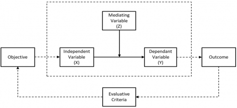
This research uses a case study approach combined with a causal model to examine the relationship between the utility management system (independent variable) and both cost efficiency and sustainability (dependent variables), with the MUT design acting as the mediating variable. Further details are outlined in sections 2.3.1 conceptual model and 2.3.2 outcome indicator and evaluative criteria.
2.3.1 Conceptual model
The Conceptual Model presents the relationships between variables, see Figure 3.
Utility Management System (UMS) (as Independent Variables) reflects two types of construction methods used in utility management, namely the traditional method and the MUT method.
MUT (as Mediating Variables) is a tunnel that co-locates more than one utility underground facilitating their subsequent repair and renewal while eliminating the need for continuous surface excavation [22]. MUT furthermore explains as follows: (1) The MUT design; (2) The vertical load scenario; (3) Space Efficiency.
Long-Term Sustainability (as Dependent Variables) divide into two aspects: (1) sustainability from a physical perspective; and (2) cost efficiency.
Figure 3. Conceptual model
2.3.2 Outcome and evaluative criteria
To assess the performance and overall impact of the proposed MUT system, several evaluative criteria and outcome indicators have been established (see Table 5).
Table 5 presents the key metrics to assess the performance and sustainability of the MUT system, focusing on system performance, sustainability, and financial performance. It outlines specific outcome indicators for each area, enabling a comparison between the MUT system and conventional methods to evaluate its long-term viability for infrastructure development in IKN Nusantara.
Table 5. Evaluative criteria and outcome indicator
|
No. |
Evaluative Criteria |
No. |
Outcome Indicator |
Unit |
|
1 |
System Performance |
1 |
Utility Integration Level |
Scale 1–5 |
|
2 |
Sustainability |
2 |
Land Use Efficiency |
% |
|
3 |
Financial Performance |
3 |
Initial Investment Cost |
Million IDR |
|
4 |
Operational Costs |
Million IDR/year |
||
|
5 |
Potential Cost Savings |
% |
This section presents the analysis of the data, focusing on the performance, efficiency, and space utilization of the MUT in comparison to conventional infrastructure. Key findings and their implications are discussed.
3.1 Results
This section presents key findings from the study, focusing on the performance, efficiency, and space utilization of the MUT system. The results are categorized into: (1) Utility Management System; (2) MUT; (3) Long-Term Sustainability.
3.1.1 Utility management system
The evaluation shows that MUT scored 5/5 for integration, indicating optimal coordination across utilities, while the traditional system scored 1 due to disorganized layouts and poor adaptability. Key findings include: (1) UMS enhanced MUT dimensional efficiency, (2) reduced utility overlap, and (3) enabled IoT-based real-time monitoring (see Table 6).
Table 6. Key advantages of MUT system over traditional systems
|
No. |
Indicator |
Value |
Interpretation |
|
1 |
Utility Integration Level |
5 |
Full integration of 5 utility types |
|
2 |
Number of Utility Types in Tunnel |
5 |
Water, wastewater, electricity, gas, fibre |
|
3 |
Monitoring Capability |
Available |
IoT-enabled infrastructure management system |
|
4 |
Maintenance Accessibility |
High |
Dedicated access paths within MUT |
|
5 |
Inter-utility Conflict Risk |
Very Low |
Centralized layout reduces overlap |
The high integration performance confirms that the Utility Management System, especially through the use of MUT, significantly enhances the MUT’s technical design, operational reliability, and long-term sustainability.
3.1.2 MUT
This section is organized into three key parts: (1) Integrating Geotechnical Data into the MUT Design, (2) Vertical Load Considerations, and (3) Enhancing Space Efficiency, each of which is explained in detail as follows:
Integrating Geotechnical Data into MUT Design. The geotechnical investigations in the KIPP IKN Nusantara region provided essential soil classification and critical data that directly influenced the structural and geometric design of the Multi-Utility Tunnel (MUT). The soil tests conducted across various zones were tied to specific design parameters, such as tunnel depth, wall support requirements, foundation type, and necessary soil improvements. Table 7 summarizes how each geotechnical test result contributed to key design decisions.
Table 7 links test results to design actions, ensuring MUT alignment avoids unstable layers, optimizes structural components, and anticipates ground behavior. For instance, weak soils in Zone 5, identified through CPT and qu tests, prompted deeper tunnels and stronger retaining materials. Modulus values from PMT and Triaxial tests informed finite element modeling, which guided the dimensioning of side walls and base slabs. These data-driven adjustments enhance tunnel performance and reduce construction risks.
The design assumes the Multi-Utility Tunnel length is 1 km (1,000 meters) for consistency with the conventional system comparison. The MUT design includes five scenarios: (1) Joint Duct Utility (JDU) “a shared duct system for various utilities like high-voltage cables and water pipes, aimed at optimizing space and reducing environmental impact.” [23, 24]; (2) Hydrant Pipe “A Hydrant Pipe is a specialized pipeline connected to the city's hydrant system, providing quick access to water for firefighting” [25]; (3) Gas Pipe is a pipeline used to transport natural gas or other gases, typically for residential, industrial, or commercial purposes [26]; (4) Joint Duct Pipe (JDP) is a channel or pipe designed to accommodate multiple types of cables or pipes within the same conduit, aimed at space efficiency and infrastructure management [27]; (5) Fiber Optic Cable (FO) functions to support high-speed telecommunication networks for internet, telephone, and data services [28, 29].
Table 7. Relationship between geotechnical tests and MUT design parameters
|
No. |
Geotechnical Test |
Key Output Parameter(s) |
Zone Applied |
Depth (m) |
Design Decision Informed |
|
1 |
Standard Penetration Test (SPT) |
N-value (relative density, bearing capacity) |
Zone 1 (West), Zone 4 (East) |
0–10 |
SPT N-value of 10–12 at 0–5 m in Zone 1 indicated loose soil; MUT placed deeper at >5 m. |
|
2 |
Cone Penetration Test (CPT) |
Tip resistance (qc), sleeve friction (fs) |
All Zones |
0–15 |
In Zone 5, qc < 5 MPa at 6 m depth signaled soft layer; tunnel depth increased to 11 m. |
|
3 |
Triaxial Test |
Shear strength, Elastic modulus (E), φ, c |
All Zones |
5–15 |
E values (450–650 kN/m²) used in PLAXIS to model stress and deformation in tunnel walls. |
|
4 |
Direct Shear Test |
Shear strength ($\tau$), cohesion (c), friction angle (φ) |
Zones 2, 3, 4 |
0–15 |
φ = 28°–30°, c = 25–40 kPa; informed base slab sizing and allowable bearing pressure. |
|
5 |
Pressure meter Test (PMT) |
Deformation modulus, pressure expansion |
Zones 3, 5 |
0–15 |
In Zone 3, pressure meter modulus >7000 kPa confirmed suitability for side wall anchoring. |
|
6 |
Oedometer Test |
Consolidation parameters (Cc, Cv) |
Zones 2, 3 |
0–10 |
Cc = 0.21, Cv = 2.3e-3 cm²/s; identified risk of settlement → soil improvement applied. |
|
7 |
Unconfined Compression Test |
Unconfined compressive strength (qu) |
Zone 5 |
0–5 |
qu = 55 kPa → shallow foundation not feasible; deep anchoring and thicker walls applied. |
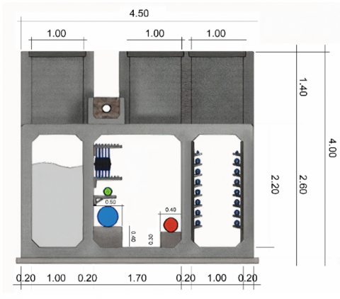
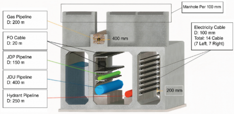
The design for IKN Nusantara is based on international best practices and is divided into three types: (1) MUT for main roads (MUT Type 1), (2) MUT for branch roads (MUT Type 2), and (3) MUT for tapping points (Tapping MUT). Figure 4 illustrates the cross-sectional diagram of a MUT, with a total width of 4.5 meters, a height of 4 meters, and a wall thickness of 0.2 meters. The effective width is 3.7 meters (after accounting for boundary walls), and the effective height is 2.6 meters (considering boundary floors) (see Figure 5).
MUT Type 1 has the following dimensions: total width of 4.5 meters, height of 4 meters, and wall thickness of 0.2 meters. The effective width is 3.7 meters (after accounting for boundary walls), and the effective height is 2.6 meters (considering boundary floors) (see Figure 5).
Figure 4. Cross-sectional diagram of the MUT Type 1
Figure 5. 3D cross-sectional view of the MUT Type 1 with utility annotations
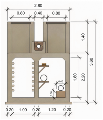
MUT Type 2 is an extension of MUT Type 1 (see Figure 6 and Figure 7).
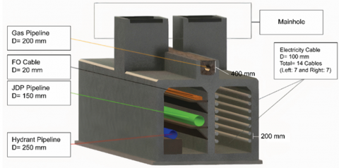
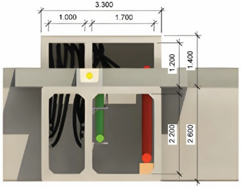
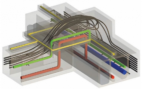
MUT Type 3 or Tapping MUT is designed for connections to the main utility tunnel, enabling utility distribution to various areas without the need for separate tunnels (see Figure 8 and Figure 9).
Figure 6. Cross-sectional diagram of MUT Type 2
Figure 7. 3D cross-sectional view of MUT Type 2
Figure 8. Top view and cross-sectional diagram of tapping MUT
Figure 9. 3D cross-sectional view of tapping MUT
The following table compares the specifications of different MUT types, including MUT Type 1, MUT Type 2, and Tapping MUT (see Table 8).
Table 9 outlines the main components of the three MUT types, detailing utilities. These components ensure efficient space usage and support essential services in urban infrastructure.
Table 8. The dimensions proposed design for MUT in IKN
|
Category |
MUT Type 1 |
MUT Type 2 |
Tapping MUT |
|
Total Width |
4.5 m |
2.80 m |
3.3 m |
|
Total Height |
4.0 m |
3.60 m |
4.0 m |
|
Chamber |
3 |
2 |
- |
|
Cross-Sectional Area of Chamber |
1 m × 2.2 m; 1.7 m × 2.2 m; 1 m × 2.2 m |
1 m × 1.8 m; 1.2 m × 1.8 m |
- |
|
Vertical Dimensions |
Manhole 1.4 m; Utilities 2.6 m |
1.4 m; 2.2 m |
- |
|
Distance Between Manholes |
100 m |
- |
- |
|
Manhole Dimensions |
1.0 m × 1.4 m × 0.80 m |
0.8 m × 1.4 m × 0.8 m |
- |
Table 9. The main components proposed design for MUT in IKN
|
Main Components |
MUT Type 1 |
MUT Type 2 |
Tapping MUT |
|
|
1 |
Joint Duct Utility (JDU) |
Diameter 400 mm |
- |
- |
|
2 |
Hydrant Pipe |
Diameter 250 mm |
Diameter 250 mm |
Diameter 250 mm |
|
3 |
Gas Pipe |
Diameter 200 mm |
Diameter 200 mm |
Diameter 200 mm |
|
4 |
Joint Duct Pipe (JDP) |
Diameter 150 mm |
Diameter 150 mm |
- |
|
6 |
Electricity Cable |
Diameter 100 mm (14 cables: 7 on left, 7 on right) |
Diameter 100 mm (14 cables: 7 on left, 7 on right) |
Diameter 100 mm (14 cables: 7 on left, 7 on right) |
|
7 |
Fibre Optic Cable (FO) |
Diameter 20 mm |
Diameter 20 mm |
Diameter 20 mm |
|
8 |
Drainage System |
Drainage Chamber (1 m × 2.6 m) |
No drainage |
No drainage |
|
9 |
Ventilation System |
Available |
Available |
Available |
To maintain consistency with traditional systems, this study focuses on MUT Type 1, designed for main roads in IKN Nusantara. It offers a more integrated solution with three chambers: (1) the Drainage Chamber for water flow, (2) the Utility Chamber for JDU, Hydrant Pipe, Gas Pipe, JDP, and Fibre Optic Cable, and (3) the Electricity Chamber for electricity cables. This design contrasts with conventional systems that require multiple separate installations and more space.
In alignment with global best practices, we will benchmark the system against successful international standards from countries like China, Japan, and the European Union [30, 31]. The MUT design varies across China, Japan, and the European Union in three key aspects: (1) China prioritizes space optimization, rapid construction, and disaster resilience with smart monitoring for improved utility management; (2) Japan focuses on seismic safety, using high-strength materials to withstand earthquakes; (3) The European Union emphasizes sustainability, energy efficiency, and minimal environmental impact, incorporating advanced monitoring and maintenance technologies.
Comparison highlights: (1) Tunnel dimensions in all regions range from 3 to 6 meters in width and 3 to 4 meters in height, with separate compartments for utilities; (2) All regions use high-strength reinforced concrete and corrosion-resistant materials for durability, especially for water and gas pipelines; (3) Structural designs: China focuses on optimization and resilience, Japan on seismic safety, and the EU on sustainability and energy efficiency; (4) Proper ventilation and drainage are ensured across all regions; (5) Utilities are separated to avoid interference, with access provided via manholes and shafts.
Vertical Load $(\mathbf{P})$. The vertical load $(\mathbf{P})$ $\left(\mathbf{k N} / \mathbf{m}^2\right)$ is divided into three as follows: Firstly, The Weight of The MUT Structural Concrete ($\boldsymbol{W}_{\boldsymbol{Concrete}}$): $\boldsymbol{W}_{\boldsymbol{Concrete}}$ refers to the weight of the concrete used in the construction of the MUT structure itself, which contributes to the overall vertical load [32]. $\boldsymbol{W}_{\boldsymbol{Concrete}}$ specific weight of concrete per square meter. It is a measure of the weight of concrete applied over an area of 1 square meter ( $\mathrm{kN} / \mathrm{m}^2$ or $\mathrm{kg} / \mathrm{m}^2$ ). $\boldsymbol{W}_{\boldsymbol {Concrete}}$ calculates as follows:
$W_{ {Concrete }}=V_{ {Concrete }} \times \rho_{ {Concrete }} \times g$ (1)
where, (1) $W_{{Concrete}}=$ Weight of the concrete per 1 meter $\left(\mathrm{kN} / \mathrm{m}^2\right)$; (2) $V_{{Concrete }}=$ specific weight of concrete per square meter $\left(k N / m^2\right), V_{{Concrete }}=b(m) \times h(m) \times t(m)$; (3) $\rho_{{Concrete }}=$ Density of the utilities $\left(\frac{\mathrm{kg}}{\mathrm{m}^3}\right)$.
Substituting the values: $\mathrm{W}_{\text {Concrete}}=(4.2 \mathrm{~m} \times 2.6 \mathrm{~m} \times$ $0.3 \mathrm{~m}) \times 25 \frac{\mathrm{kN}}{\mathrm{m}^3}=3.276 \mathrm{~m}^3 \times 25 \frac{\mathrm{kN}}{\mathrm{m}^3}=81.9 \mathrm{kN}$. The density of the concrete is already expressed in kN/m³ (kilonewtons per cubic meter), which inherently includes the effect of gravity. Therefore, there is no need to multiply by gravitational acceleration (9.81 m/s²).
Secondly, the Load of the Utilities ($\mathrm{W}_{\text {utility}}$): $\mathrm{W}_{\text {utility}}$ represents the load generated by the utilities within the MUT, including pipes, cables, and other equipment actively used during operation. The total weight of utilities ($\mathrm{W}_{\text {utility}}$) is calculated by summing the individual weights of each utility system installed in the tunnel. The formula is as follows:
$\begin{gathered}\mathrm{W}_{\text {utility }}=\mathrm{W}_{\mathrm{JDU}}+\mathrm{W}_{\mathrm{H}}+\mathrm{W}_{\mathrm{GP}}+\mathrm{W}_{\mathrm{JDP}}+\mathrm{W}_{\mathrm{EC}}+\mathrm{W}_{\mathrm{D}}+\mathrm{W}_{\mathrm{V}}+\mathrm{W}_{\mathrm{FO}}\end{gathered}$ (2)
where, (1) $\mathrm{W}_{\text {utility }}$ = total weight of utilities within the MUT (kN/m²); (2) $\mathrm{W}_{\mathrm{JDU}}$= wiegth of Joint Duct Utility (kN/m²); (3) $\mathrm{W}_{\mathrm{H}}$= weight of Hydrant Pipe (kN/m²); (4) $\mathrm{W}_{\mathrm{GP}}$= Gas Pipe (kN/m²); (5) $\mathrm{W}_{\mathrm{JDP}}$= weight of Joint Duct Pipe (kN/m²); (6) $\mathrm{W}_{\mathrm{EC}}$= Weight of Electricity Cable (kN/m²); (7) $\mathrm{W}_{\mathrm{D}}$ = Drainage Contains (kN/m²); (8) $\mathrm{W}_{\mathrm{V}}$= Ventilation Contains (kN/m²); (9) $\mathrm{W}_{\mathrm{FO}}$= weight of Fibre Optic (kN/m²).
Substituting the values: $\quad W_{{utility }}=17.035+10.630+6.791+3.822+4.245+0.95+0.95+0.577=45 \mathrm{kN} / \mathrm{m}$.
Lastly, Total Vertical Loads ($P$) per meter length (kN/m²) are calculated as follows:
$\mathrm{P}=\mathrm{W}_{\text {Concrete}}+\mathrm{W}_{\text {utility}}$ (3)
where, (1) $\mathrm{P}=$ Total vertical loads $\left(\mathrm{kN} / \mathrm{m}^2\right)$; (2) $\mathrm{W}_{\text {Concrete}}=$ specific weight of concrete per square meter ($\mathrm{kN} / \mathrm{m}^2$); (3) $\mathrm{W}_{\text {utilitas}}=$ Weight of utility inside the MUT ($\mathrm{kN} / \mathrm{m}^2$).
Substituting the values: $P=W_{ {Concrete}}+W_{{utilitas }}=81.9 \frac{\mathrm{kN}}{\mathrm{m}}+45 \frac{\mathrm{kN}}{\mathrm{m}}=126.9 \frac{\mathrm{kN}}{\mathrm{m}}$. In other words, for every square meter of MUT, the vertical load $(P)$ is $126.9 \frac{\mathrm{kN}}{\mathrm{m}^2}$.
Space Efficiency. Relative space efficiency is calculated using the ratio between the MUT (Multi Utility Tunnel) system and the conventional system by comparing the total space used by each system, as formulated in Eq. (4) as follows:
$R_e=\frac{L_{ {Conventional }}-L_{M U T}}{L_{{Conventional }}} \times 100 \%$ (4)
where, (1) $R_e$= Relative space efficiency (in percentage); (2) $L_{Conventional}$= Total utility space length in the conventional system (in meters); (3) $L_{M U T}$= Total utility space length in the MUT system (in meters).
Yielding the following value: $\begin{aligned} \mathrm{R}_{\mathrm{e}}=\frac{\mathrm{L}_{\text {Conventional }}-\mathrm{L}_{\mathrm{MUT}}}{\mathrm{L}_{\text {Conventional }}} \times 100 \%=\frac{7.5 \text { meter }-4.5 \text { meter }}{7.5 \text { meter }} \times 100 \%=40 \%\end{aligned}$. The MUT system can save up to 40% of space (Re = 40%) compared to conventional methods.
The value of $R_e$ indicates the level of efficiency of the new system compared to the conventional system, as follows: (1) $R_e$ > 1: The new design is less efficient, using more space than the conventional design (space wasted); (2) $R_e$ = 1: The new design and conventional design are equally efficient, with no space saving; (3) $R_e$ < 1: The new design (MUT) is more efficient, saving space compared to the conventional design.
3.1.3 Long-term sustainability (dependent variables)
Long-term sustainability divides into two aspects: (1) sustainability from a physical perspective; and (2) cost efficiency.
Sustainability from a physical perspective can be viewed from two aspects: (1) Soil Stability and (2) Structural Stability. The explanations for each are as follows: Firstly, Soil Stability analyse using three 3 parameters which is Modulus Elasticity (E), Poisson's Ratio (ν), Maximum Stress ($\sigma_{\max }$) [33]. First, the explanation regarding soil stability is addressed through Modulus of Elasticity (E). Modulus of Elasticity (E) is used to measure the stiffness of the soil, providing insights into how much the soil can deform under stress [34, 35]. Reference [36] indicates the soil’s ability to resist elastic deformation (Ɛ) when subjected to stress ($\sigma$) [37]. The higher the soil stiffness (E), the smaller the elastic deformation (Ɛ), which indicates better stability [32, 38] (see Eq. (5)).
$\varepsilon=\frac{\sigma}{\mathrm{E}}$ (5)
where, (1) $\varepsilon=$ the ratio of the change in length $(\Delta L)$ to the original length $(L)$, or $\frac{\Delta L}{L}$; (2) $\sigma=$ force per unit area (kN/m²) or Pascal (Pa); (3) $E=$ modulus of elasticity.
In this research, Modulus of Elasticity (E) measured using Triaxial Test and Cone Penetration Test [39, 40]. Table 10 summarizes the elastic modulus (E), tested stress $\left(\sigma_{ {Test }}\right)$, and calculated stress $\left(\sigma_{ {calc }}\right)$ for various soil types at different depths in the KIPP zones.
Table 9 highlights key findings:
(1) Elastic Modulus (E) increases with depth, ranging from 500-600 kN/m² in West KIPP and 550-650 kN/m² in South KIPP;
(2) Test Stress $\left(\sigma_{ {Test }}\right)$ is higher in denser soils, e.g., 200 kN/m² in clayey sand to 250 kN/m² in compact sand in West KIPP;
(3) $\sigma_{{Test }}$ and $\sigma_{ {calc }}$ are consistent, validating the model;
(4) Relative Deformation (Ɛ) increases slightly with depth but remains within limits, with denser soils deforming less;
(5) Soil type significantly affects mechanical properties, with denser soils showing higher E and $\sigma_{{Test }}$ values.
Table 10. Elastic modulus, tested stress, and calculated stress for various soil types in KIPP zones
|
No. |
Location |
Depth (m) |
Soil Types |
Modulus Elasticity (E) |
$\sigma_{{Test }}$ (kN/m²) |
||||
|
$E_{{Test }}$ (kN/m²) |
$L_{{Test }}$ (m) |
ΔL (mm) |
Ɛ (ΔL/ L) |
$\sigma_{calc}$ (kN/m²) |
|||||
|
1 |
West KIPP (KIPP Zone 1) |
0 - 5 |
Clayey Sand |
500 |
10 |
4000 |
0.4 |
200 |
200 |
|
5-10 |
Compact Clayey Sand |
550 |
10 |
4000 |
0.4 |
220 |
220 |
||
|
10-15 |
Compact Sand |
600 |
10 |
4200 |
0.42 |
250 |
250 |
||
|
2 |
North KIPP (KIPP Zone 2) |
0 - 5 |
Fine Sand-Clay |
480 |
10 |
3800 |
0.38 |
180 |
180 |
|
5-10 |
Compact Sand |
520 |
10 |
3800 |
0.38 |
200 |
200 |
||
|
10-15 |
Compact Sand |
580 |
10 |
4100 |
0.41 |
240 |
240 |
||
|
3 |
South KIPP (KIPP Zone 3) |
0 - 5 |
Sandy Clay |
550 |
10 |
4500 |
0.45 |
250 |
250 |
|
5-10 |
Compact Clay |
600 |
10 |
4700 |
0.47 |
280 |
280 |
||
|
10-15 |
Sandy Clay-Gravel |
650 |
10 |
4800 |
0.48 |
300 |
300 |
||
|
4 |
East KIPP (KIPP Zone 4) |
0-5 |
Fine Sand |
450 |
10 |
3600 |
0.36 |
160 |
160 |
|
5-10 |
Fine Sand-Clay |
500 |
10 |
3600 |
0.36 |
180 |
180 |
||
|
10-15 |
Clayey Sand |
550 |
10 |
4000 |
0.4 |
200 |
200 |
||
|
5 |
Central KIPP (KIPP Zone 5) |
0-5 |
Gravelly Sand |
400 |
10 |
3500 |
0.35 |
140 |
140 |
|
5-10 |
Compact Sand-Gravel |
480 |
10 |
3300 |
0.33 |
160 |
160 |
||
|
10-15 |
Compact Sand |
550 |
10 |
3600 |
0.36 |
200 |
200 |
||
Second, the explanation regarding soil stability is addressed through Poisson's Ratio (ν). Poisson's Ratio (ν) measures the ratio of lateral to axial strain under stress and is crucial for assessing lateral pressure and volumetric deformation in soils [41, 42]. A high ν (near 0.5) indicates nearly incompressible saturated soils, while lower values (0.2–0.3) suggest better stability in granular soils. It’s determined via lab tests like Triaxial and Uniaxial Compression. For this study, a soil length of 10 m (L) is assumed to calculate deformation. Table 11 lists ν and Elastic Modulus (E) values across KIPP zones, essential for evaluating soil stability and MUT design suitability.
Table 11. Elastic Modulus (E) and Poisson's Ratio (ν) for various soil types in the KIPP zones
|
No |
Location |
Depth (m) |
Soil Types |
$E_{{Test }}\left(\mathbf{k N} / \mathbf{m}^2\right)$ |
Poisson Ratio (ν) |
|
1 |
West KIPP (KIPP Zone 1) |
0 - 5 |
Clayey Sand |
500 |
0.30 |
|
0 - 5 |
Compact Clayey Sand |
550 |
0.31 |
||
|
5-10 |
Compact Sand |
600 |
0.32 |
||
|
2 |
North KIPP (KIPP Zone 2) |
10-15 |
Fine Sand-Clay |
480 |
0.29 |
|
0 - 5 |
Compact Sand |
520 |
0.30 |
||
|
5-10 |
Compact Sand |
580 |
0.32 |
||
|
3 |
South KIPP (KIPP Zone 3) |
10-15 |
Sandy Clay |
550 |
0.31 |
|
0 - 5 |
Compact Clay |
600 |
0.32 |
||
|
5-10 |
Sandy Clay-Gravel |
650 |
0.33 |
||
|
4 |
East KIPP (KIPP Zone 4) |
10-15 |
Fine Sand |
450 |
0.28 |
|
0 - 5 |
Fine Sand-Clay |
500 |
0.29 |
||
|
5-10 |
Clayey Sand |
550 |
0.30 |
||
|
5 |
Central KIPP (KIPP Zone 5) |
10-15 |
Gravelly Sand |
400 |
0.27 |
|
0 - 5 |
Compact Sand-Gravel |
480 |
0.30 |
||
|
5-10 |
Compact Sand |
550 |
0.31 |
Based on Table 10, Poisson’s Ratio (ν) and Elastic Modulus (E) generally increase with depth across all KIPP zones. For instance, in West KIPP (Zone 1), ν rises slightly from 0.30 to 0.32 while E increases from 500 to 600 kN/m². Similar upward trends are observed in North, South, East, and Central KIPP zones, with denser soils consistently showing higher values. This indicates a positive correlation between Poisson’s Ratio and Elastic Modulus, where denser soils exhibit greater elasticity and reduced deformation under stress.
Thirdly, the explanation regarding soil stability is addressed through Maximum Stress $\left(\sigma_{\max }\right)$. Maximum Stress $\left(\sigma_{\max }\right)$ represents the maximum stress the soil can withstand before failure, essential for understanding the soil’s load-bearing capacity. It directly evaluates soil bearing capacity and defines the safe load limit for structures like MUT, ensuring stability. Measured through Direct Shear, Triaxial, or Unconfined Compression Tests.
$\sigma_{\max }=\frac{\text { Force }(\mathrm{N})}{\text { Area }\left(\mathrm{m}^2\right)}$ (6)
where, (1) $\text {Force}$ = total external load or force applied to the soil $(\mathrm{N})$ (taken from test result. Force (N) $=\sigma_{\max } \times$ Area $\left(\mathrm{m}^2\right)$ $\times 1000$ (1000 is the conversion factor from kPa to N/m² (1 kPa = 1000 N/m²)); (2) $\text {Area}$ = contact area between the soil and the applied force $\left(\mathrm{m}^2\right)$. Contact area assume for 10.92 m² for soil loading analysis. Maximum Stress $\left(\sigma_{\max }\right)$ presented in Table 12.
Table 12. Data of maximum stress, force, and area for various soil types in different test zones
|
No |
Location |
Depth (m) |
Soil Types |
Maximum Stress ($\sigma_{M a x}$) |
||
|
$\sigma_{M a x}$ (kN/m²) |
Force (N) |
Area (m²) |
||||
|
1 |
West KIPP (KIPP Zone 1) |
0 - 5 |
Clayey Sand |
200 |
2,184,000 |
10.92 |
|
5-10 |
Compact Clayey Sand |
220 |
2,402,400 |
10.92 |
||
|
10-15 |
Compact Sand |
250 |
2,730,000 |
10.92 |
||
|
2 |
North KIPP (KIPP Zone 2) |
0 - 5 |
Fine Sand-Clay |
180 |
1,965,600 |
10.92 |
|
5-10 |
Compact Sand |
200 |
2,184,000 |
10.92 |
||
|
10-15 |
Compact Sand |
240 |
2,620,800 |
10.92 |
||
|
3 |
South KIPP (KIPP Zone 3) |
0 - 5 |
Sandy Clay |
250 |
2,730,000 |
10.92 |
|
5-10 |
Compact Clay |
280 |
3,058,800 |
10.92 |
||
|
10-15 |
Sandy Clay-Gravel |
300 |
3,276,000 |
10.92 |
||
|
4 |
East KIPP (KIPP Zone 4) |
0 - 5 |
Fine Sand |
160 |
1,747,200 |
10.92 |
|
5-10 |
Fine Sand-Clay |
180 |
1,965,600 |
10.92 |
||
|
10-15 |
Clayey Sand |
200 |
2,184,000 |
10.92 |
||
|
5 |
Central KIPP (KIPP Zone 5) |
0 - 5 |
Gravelly Sand |
140 |
1,526,400 |
10.92 |
|
5-10 |
Compact Sand-Gravel |
160 |
1,747,200 |
10.92 |
||
|
10-15 |
Compact Sand |
200 |
2,184,000 |
10.92 |
||
Table 12 shows that maximum stress (σmax) increases with depth across all KIPP zones. In West KIPP (Zone 1), Sand-Clay soil stress rises from 200 kPa at 0-5 m to 250 kPa at 10-15 m. North KIPP (Zone 2) follows a similar trend, increasing from 180 kPa to 240 kPa. South KIPP (Zone 3) has the highest stress values, reaching 300 kPa at 10-15 m, indicating stronger soil suitable for heavier structures.
East (Zone 4) and Central KIPP (Zone 5) show lower stress levels, with gravelly soils having the lowest bearing capacity, requiring reinforcement or design adjustments.
Secondly, sustainability from a physical perspective can be assessed through structural stability, which refers to a structure's ability to endure loads and forces without failure, deformation, or collapse [43, 44]. To analyse structural stability, three key factors are considered: (1) Total Stress ($\sigma_{t o t}$); (2) Maximum Deformation (∆); and (3) Safety Factor (FS).
First, sustainability from a physical perspective can be assessed through structural stability using the indicator of Total Stress ($\sigma_{\text {tot}}$). Total Stress ($\sigma_{\text {tot}}$) applied to the soil by structural elements above it. Total stress ($\sigma_{\text {tot}}$) results from external loads. It is calculated using Eq. (7):
$\sigma_{t o t}=\frac{\mathrm{P}}{\mathrm{A}}$ (7)
where, (1) $\sigma_{t o t}=$ Total stress $(\mathrm{kPa})$; (2) $P=$ Vertical load $\left(\mathrm{kN} / \mathrm{m}^2\right) ;(3) A=$ Base area of the structure ($\mathrm{m}^2$).
Total Stress on soil by test ($\sigma_{\text {Test}}$). Total Stress determined through tests such as the Direct Shear Test, Triaxial Test, or Unconfined Compression Test [45, 46]. It is used to assess soil stability by comparing the applied pressure to the soil's bearing capacity. If the total stress $\sigma_{tot}>\sigma_{Test}$, the soil risks being overloaded and may fail, requiring reinforcement for safe MUT support. If $\sigma_{\text {tot }}<\sigma_{{Test}}$, the soil has higher bearing capacity than tested, offering potential cost savings in foundation design. When $\sigma_{\text {tot }}=\sigma_{{Test}}$, the soil is stable, confirming it can safely bear the expected loads and ensuring reliable MUT foundation design (see Table 13).
Table 13. Soil stability evaluation based on total stress $\left(\sigma_{t o t}\right)$ and test stress $\left(\sigma_{Test}\right)$ comparison across KIPP zones
|
No. |
Location |
Depth (m) |
Soil Types |
P (kN/m²) |
A (m²) |
$\sigma_{t o t}$ (kN/m²) |
$\sigma_{Test}$ (kN/m²) |
Evaluation |
|
1 |
West KIPP (KIPP Zone 1) |
0 - 5 |
Clayey Sand |
126.9 |
10.92 |
11.62 |
200 |
${\sigma}_{{tot }}$ < ${\sigma}_{{Test}}$ |
|
0 - 5 |
Compact Clayey Sand |
126.9 |
10.92 |
11.62 |
220 |
${\sigma}_{{tot }}$ < ${\sigma}_{{Test}}$ |
||
|
5-10 |
Compact Sand |
126.9 |
10.92 |
11.62 |
250 |
${\sigma}_{{tot }}$ < ${\sigma}_{{Test}}$ |
||
|
2 |
North KIPP (KIPP Zone 2) |
10-15 |
Fine Sand-Clay |
126.9 |
10.92 |
11.62 |
180 |
${\sigma}_{{tot }}$ < ${\sigma}_{{Test}}$ |
|
0 - 5 |
Compact Sand |
126.9 |
10.92 |
11.62 |
200 |
${\sigma}_{{tot }}$ < ${\sigma}_{{Test}}$ |
||
|
5-10 |
Compact Sand |
126.9 |
10.92 |
11.62 |
240 |
${\sigma}_{{tot }}$ < ${\sigma}_{{Test}}$ |
||
|
3 |
South KIPP (KIPP Zone 3) |
10-15 |
Sandy Clay |
126.9 |
10.92 |
11.62 |
250 |
${\sigma}_{{tot }}$ < ${\sigma}_{{Test}}$ |
|
0 - 5 |
Compact Clay |
126.9 |
10.92 |
11.62 |
280 |
${\sigma}_{{tot }}$ < ${\sigma}_{{Test}}$ |
||
|
5-10 |
Sandy Clay-Gravel |
126.9 |
10.92 |
11.62 |
300 |
${\sigma}_{{tot }}$ < ${\sigma}_{{Test}}$ |
||
|
4 |
East KIPP (KIPP Zone 4) |
10-15 |
Fine Sand |
126.9 |
10.92 |
11.62 |
160 |
${\sigma}_{{tot }}$ < ${\sigma}_{{Test}}$ |
|
0 - 5 |
Fine Sand-Clay |
126.9 |
10.92 |
11.62 |
180 |
${\sigma}_{{tot }}$ < ${\sigma}_{{Test}}$ |
||
|
5-10 |
Clayey Sand |
126.9 |
10.92 |
11.62 |
200 |
${\sigma}_{{tot }}$ < ${\sigma}_{{Test}}$ |
||
|
5 |
Central KIPP (KIPP Zone 5) |
10-15 |
Gravelly Sand |
126.9 |
10.92 |
11.62 |
140 |
${\sigma}_{{tot }}$ < ${\sigma}_{{Test}}$ |
|
0 - 5 |
Compact Sand-Gravel |
126.9 |
10.92 |
11.62 |
160 |
${\sigma}_{{tot }}$ < ${\sigma}_{{Test}}$ |
||
|
5-10 |
Compact Sand |
126.9 |
10.92 |
11.62 |
200 |
${\sigma}_{{tot }}$ < ${\sigma}_{{Test}}$ |
As the conclusion on the analysis of total stress ($\sigma_{t o t}$) and field test results ($\sigma_{{Test}}$) across various KIPP zones, the following conclusions can be drawn: In all KIPP zones, total stress ($\sigma_{\text {t o t}}$) is consistently lower than tested stress ($\sigma_{\text {Test}}$), indicating that soil strength exceeds laboratory test results. This confirms soil stability across all zones, meaning the soil can safely support applied loads. Consequently, structural designs can be more efficient with less need for reinforcement, and the soil may support greater loads if required in the future.
Second, sustainability from a physical perspective can be assessed through structural stability using the indicator of Maximum Deformation ($\Delta$). Maximum Deformation ($\Delta$) is the change in shape (strain) of the soil due to the stress applied by vertical loads This parameter is used to assess the stability of the soil beneath structures and utilities. It is calculated using Eq. (8):
$\Delta=\frac{P . L}{E . A}$ (8)
where, (1) $\Delta$ = Maximum deformation (m); (2) $P$ = Vertical load ($\mathrm{kN} / \mathrm{m}^2$); (3) $L$ = Length of the soil element (m); (4) $E$ = Soil stiffness (kPa); (5) $A$ = Cross-sectional area of the soil element ($\mathrm{m}^2$). The Maximum Deformation ($\Delta$) results are presented in Table 14.
Table 14. Soil characteristics by zone and depth at KIPP
|
No. |
Location |
Depth (m) |
Soil Types |
P (kN/m²) |
A (m²) |
E (kN/m²) |
L (m) |
(∆) (m) |
|
1 |
West KIPP (KIPP Zone 1) |
0 - 5 |
Clayey Sand |
126.9 |
10.92 |
500 |
10 |
0.026 |
|
5-10 |
Compact Clayey Sand |
126.9 |
10.92 |
550 |
10 |
0.023 |
||
|
10-15 |
Compact Sand |
126.9 |
10.92 |
600 |
10 |
0.021 |
||
|
2 |
North KIPP (KIPP Zone 2) |
0 - 5 |
Fine Sand-Clay |
126.9 |
10.92 |
480 |
10 |
0.024 |
|
5-10 |
Compact Sand |
126.9 |
10.92 |
520 |
10 |
0.022 |
||
|
10-15 |
Compact Sand |
126.9 |
10.92 |
580 |
10 |
0.021 |
||
|
3 |
South KIPP (KIPP Zone 3) |
0 - 5 |
Sandy Clay |
126.9 |
10.92 |
550 |
10 |
0.026 |
|
5-10 |
Compact Clay |
126.9 |
10.92 |
600 |
10 |
0.022 |
||
|
10-15 |
Sandy Clay-Gravel |
126.9 |
10.92 |
650 |
10 |
0.020 |
||
|
4 |
East KIPP (KIPP Zone 4) |
0 - 5 |
Fine Sand |
126.9 |
10.92 |
450 |
10 |
0.027 |
|
5-10 |
Fine Sand-Clay |
126.9 |
10.92 |
500 |
10 |
0.024 |
||
|
10-15 |
Clayey Sand |
126.9 |
10.92 |
550 |
10 |
0.022 |
||
|
5 |
Central KIPP (KIPP Zone 5) |
0 - 5 |
Gravelly Sand |
126.9 |
10.92 |
400 |
10 |
0.031 |
|
5-10 |
Compact Sand-Gravel |
126.9 |
10.92 |
480 |
10 |
0.024 |
||
|
10-15 |
Compact Sand |
126.9 |
10.92 |
550 |
10 |
0.021 |
Table 14 shows Maximum Deformation (∆) for various soil types across five KIPP zones, factoring in vertical load (P), cross-sectional area (A), elasticity modulus (E), and soil length (L). Soils with higher elasticity, like Compact Sand and Clay, exhibit smaller deformations, indicating better stability, while Fine Sand and Gravel show larger deformations, signaling vulnerability. For example, Gravelly Sand in Zone 5 has ∆=0.031 m, higher than Fine Sand in Zone 4 (∆=0.022 m). Maximum Deformation is crucial for structural stability as higher deformation reduces soil bearing capacity and increases settlement risk.
Third, sustainability from a physical perspective can be assessed through structural stability using the indicator of Safety Factor (FS). Safety Factor (FS) is the ratio between the soil's maximum stress ($\sigma_{\max}$) assume equal ($\sigma_{{Test}}$) and the total stress ($\sigma_{\text {t o t}}$) assume equal applied by the structural load [47-49]. The formula is:
$F S=\frac{\sigma_{\max }}{\sigma_{t o t}}$ (9)
Interpretation of results is as follows: (1) FS > 1.5 (Safe) – The soil is sufficiently stable to support the load; (2) FS = 1.0 (Marginal) – The soil is close to its stability limit and requires attention; (3) FS < 1.0 (Unsafe) – The soil is unstable and at risk of failure. Safety Factor (FS) results are presented in Table 15.
Table 15. Safety Factor (FS) for different zones and soil types
|
No. |
Location |
Depth (m) |
Soil Types |
$\sigma_{\max } / \sigma_{{Test }}$ |
P/ $\sigma_{{tot}}$ |
FS |
Interpretation |
|
1 |
West KIPP (KIPP Zone 1) |
0 - 5 |
Clayey Sand |
200 |
126.9 |
1.57 |
Soil is safe and can withstand the applied stress. |
|
5-10 |
Compact Clayey Sand |
220 |
126.9 |
1.73 |
Soil is safe and can withstand the applied stress. |
||
|
10-15 |
Compact Sand |
250 |
126.9 |
1.97 |
Soil is safe and can withstand the applied stress. |
||
|
2 |
North KIPP (KIPP Zone 2) |
0 - 5 |
Fine Sand-Clay |
180 |
126.9 |
1.42 |
Soil is safe and can withstand the applied stress. |
|
5-10 |
Compact Sand |
200 |
126.9 |
1.57 |
Soil is safe and can withstand the applied stress. |
||
|
10-15 |
Compact Sand |
240 |
126.9 |
1.89 |
Soil is safe and can withstand the applied stress. |
||
|
3 |
South KIPP (KIPP Zone 3) |
0 - 5 |
Sandy Clay |
250 |
126.9 |
1.97 |
Soil is safe and can withstand the applied stress. |
|
5-10 |
Compact Clay |
280 |
126.9 |
2.21 |
Soil is safe and can withstand the applied stress. |
||
|
10-15 |
Sandy Clay-Gravel |
300 |
126.9 |
2.36 |
Soil is safe and can withstand the applied stress. |
||
|
4 |
East KIPP (KIPP Zone 4) |
0 - 5 |
Fine Sand |
160 |
126.9 |
1.26 |
Soil is safe and can withstand the applied stress. |
|
5-10 |
Fine Sand-Clay |
180 |
126.9 |
1.42 |
Soil is safe and can withstand the applied stress. |
||
|
10-15 |
Clayey Sand |
200 |
126.9 |
1.57 |
Soil is safe and can withstand the applied stress. |
||
|
5 |
Central KIPP (KIPP Zone 5) |
0 - 5 |
Gravelly Sand |
140 |
126.9 |
1.10 |
Soil may not withstand the applied load and is at risk of structural failure. |
|
5-10 |
Compact Sand-Gravel |
160 |
126.9 |
1.26 |
Soil is safe and can withstand the applied stress. |
||
|
10-15 |
Compact Sand |
200 |
126.9 |
1.57 |
Soil is safe and can withstand the applied stress. |
The Safety Factor (FS) analysis across KIPP zones indicates that most soils, particularly in West, North, South, and East KIPP, can support applied loads safely, with FS values above 1. South KIPP (Zone 3) exhibits the highest stability (FS = 2.36), while East KIPP (Zone 4) also shows safe FS values ranging from 1.26 to 1.57. However, Central KIPP (Zone 5), particularly the Gravelly Sand at 0-5 m depth, has a marginal FS of 1.10, indicating a higher risk of structural failure. This highlights the need for soil improvement or design modifications in Central KIPP to ensure stability and prevent failure.
Structural analysis confirms that most KIPP soils can bear applied loads, with bearing capacities surpassing lab assumptions. Soils with higher elasticity, such as compact sand and clay, deform less and exhibit better stability. Conversely, fine and gravelly sands deform more, which could pose risks if unsterilized. While the majority of zones exhibit FS values greater than 1, Central KIPP’s FS of 1.10 signals potential failure risks and the necessity for reinforcement. Therefore, most zones are suitable for MUT construction, with Central KIPP requiring soil strengthening for secure foundations.
Long-term sustainability, in terms of cost efficiency, can be assessed through Total Cost and Asset Depreciation. Total Cost (∆C) combines Capital Expenditure (Capex) and Operational Expenditures (Opex) for both the traditional and MUT systems, as defined in Eq. (7).
$\Delta C=C_{ {Capex }}+C_{{Opex }}$ (10)
where, (1) $C_{ {Capex}}$ = Capex (IDR); (2) $C_{{Opex}}$ = Opex (IDR).
Firstly, long-term sustainability in terms of cost efficiency assessed through aspects of $C_{ {Capex}}$ as part of the total cost. $C_{ {Capex}}$ refers to the funds spent to acquire, upgrade, or maintain physical assetss [50]. In this research, $C_{ {Capex}}$ is measured per 1,000 meters. $\mathrm{C}_{\text {Capex}}$ calculated by summing all costs incurred during the construction of both systems (see Eq. (11)).
$\begin{aligned} C_{{Capex }}=C_{J D U}+ & C_H+C_{G P}+C_{J D P}+C_{E C}+C_D +C_{F O}+C_{E C}+C_{C C}\end{aligned}$ (11)
where, (1) JDU installation cost ($C_{J D U}$) (IDR); (2) Hydrant cost ($C_H$) (IDR); (3) Gas Pipe cost ($C_{G P}$) (IDR); (4) JDP cost ($C_{J D P}$) (IDR); (5) Electricity Cable cost ($C_{E C}$) (IDR); (6) Drainage cost ($C_D$); (7) FO $\left(C_{F O}\right)$. Plus, two additional new costs, namely: (8) Excavation (5 lanes) Cost ($C_{E C}$) (IDR); and (9) Construction Cost ($C_{C C}$) Excavation (5 lanes) Cost (IDR).
Capex efficiency (CEE) between the traditional system and MUT is calculated using the following equation.
$C E E=\frac{C_{{Capex\ Traditional }}-C_{{Capex\ MUT }}}{C_{ {Capex\ Traditional }}} \times 100 \%$ (12)
where, (1) $CEE$ (IDR); (2) $C_{Capex\ Traditional}$ (IDR); (3) $C_{{Capex\ MUT}}$ (IDR).
The Capex for both methods is presented in Table 16.
Table 16. Capex for conventional and MUT methods
|
No. |
Items |
Diameter (m) |
Length (m) |
Conventional |
MUT |
||
|
Price (IDR) |
$C_{ {Construction }}$ per Kilometres |
Price (IDR) |
$C_{ {Construction }}$ per Kilometres |
||||
|
1 |
JDU |
400 mm |
1000 |
- |
- |
2.000.000 |
2.000.000.000 |
|
2 |
Hydrant |
250 mm |
1000 |
2.500.000 |
2.500.000.000 |
2.500.000 |
2.500.000.000 |
|
3 |
Gas Pipe |
200 mm |
1000 |
1.500.000 |
1.500.000.000 |
1.500.000 |
1.500.000.000 |
|
4 |
JDP |
150 mm |
1000 |
1.000.000 |
1.000.000.000 |
1.000.000 |
1.000.000.000 |
|
5 |
Electricity Cable |
100 mm |
1000 |
- |
- |
- |
- |
|
6 |
Drainage |
|
1000 |
500.000 |
500.000.000 |
- |
- |
|
7 |
Fiber Optic |
20 mm |
1000 |
750.000 |
750.000.000 |
750.000 |
750.000.000 |
|
8 |
Excavation (5 lanes) |
|
1000 |
500.000 |
2.500.000.000 |
- |
- |
|
9 |
MUT Construction |
4.5 m × 4 m |
1000 |
- |
- |
5.500.000 |
5.500.000.000 |
|
Capital Expenditures |
8.750.000.000 |
|
13.250.000.000 |
||||
Long-term sustainability in terms of cost efficiency assessed through aspects of $\mathrm{C}_{\mathrm{Opex}}$ as part of the total cost. $\mathrm{C}_{\mathrm{Opex}}$ refers to the ongoing, recurring costs incurred during the operation an infrastructure or system after its construction [50]. The operational costs of each utility calculate as follows (see Eq. (13)).
$\begin{gathered}C_{{Opex }}=O_{J D U}+O_H+O_{G P}+O_{J D P}+O_{E C}+O_D +O_{F O}+O_{U M}\end{gathered}$ (13)
where, (1) JDU cost $\left(O_{J D U}\right)$ (IDR); (2) Hydrant cost $\left(O_H\right)$ (IDR); (3) Gas Pipe cost ($O_{G P}$) (IDR); (4) JDP cost ($O_{J D P}$) (IDR); (5) Electricity Cable cost ($O_{E C}$) (IDR); (6) Drainage cost $\left(O_D\right)$ (IDR); (7) FO $\left(O_{F O}\right)$ (IDR). Plus, one additional new cost; (8) utility maintenance cost ($O_{U M}$) (IDR).
The calculation of $C_{{Opex }}$ efficiency (OEE) between the traditional system and MUT is calculated using the following equation:
$OEE =\frac{C_{{Opex\ Traditional }}-C_{{Opex\ MUT}}}{C_{{Opex\ Traditional }}} \times 100 \%$ (14)
where, (1) $OEE$ (IDR); (2) $C_{{Opex\ Traditional}}$ (IDR); (3) $C_{{Opex\ MUT}}$ (IDR).
If the value of CEE MUT or OEE MUT is positive, it indicates that the MUT method is more cost-efficient compared to the conventional method, and the other way around. The Opex for both methods are presented in Table 17.
As summary, the total costs over a 10-year period are summarized in Table 18.
Secondly, long-term sustainability in term of cost efficiency can be assessed through aspects of Asset Depreciation. Asset depreciation is the systematic allocation of the initial cost of a fixed asset used in an entity’s operations over its useful life. Depreciation reflects the decrease in asset value over time due to wear and tear, damage, usage, or other external factors [51].
Table 17. $C_{{Opex}}$ for conventional and MUT methods
|
No. |
Items |
Diameter (m) |
Length (m) |
Conventional Methods |
MUT |
||
|
Price (IDR) |
Per Kilometres |
Price (IDR) |
Per Kilometres |
||||
|
1 |
JDU |
400 mm |
1000 |
- |
- |
75.000 |
75.000.000 |
|
2 |
Hydrant |
250 mm |
1000 |
250.000 |
250.000.000 |
75.000 |
75.000.000 |
|
3 |
Gas |
200 mm |
1000 |
100.000 |
100.000.000 |
40.000 |
40.000.000 |
|
4 |
JDP |
150 mm |
1000 |
100.000 |
100.000.000 |
40.000 |
40.000.000 |
|
5 |
Electricity Cable |
100 mm |
1000 |
- |
- |
- |
- |
|
6 |
Fibre Optic |
20 mm |
1000 |
50.000 |
50.000.000 |
25.000 |
25.000.000 |
|
7 |
Drainage |
|
1000 |
50.000 |
50.000.000 |
- |
- |
|
8 |
Operational |
|
1000 |
- |
- |
47.500 |
47.500.000 |
|
Operational Costs |
550.000.000 |
|
302.500.000 |
||||
Table 18. A comparison of cost parameters and efficiency between the conventional method and the MUT system
|
No |
Parameter |
Conventional (IDR) |
MUT (IDR) |
|
1 |
$C_{{Capex}}$ |
8.750.000.000 |
13.250.000.000 |
|
2 |
$C_{{Opex}}$ |
550.000.000 |
302.500.000 |
|
3 |
Total Maintenance Over 10 Years (45%) |
5.500.000.000 |
3.025.000.000 |
|
4 |
Total 10-Year Cost |
14.250.000.000 |
16.275.000.000 |
|
5 |
Space Savings (40%) |
None |
3.500.000.000 |
|
6 |
Total Effective Cost (after Space Savings) |
14.250.000.000 |
12.775.000.000 |
Depreciation is calculated using the Straight-Line Method [52], see equation as follows:
$A D=\frac{C_{{Capex }}-R V}{U L}$ (15)
where, (1) Annual Depreciation (AD) = asset value decreases each year (IDR); (2) $C_{Capex}$ is the cost of building or purchasing the asset (IDR); (3) Residual Value (RV) is the expected value remaining after the asset’s useful life (IDR); (4) Useful Life (UL) is the duration the asset is expected to be in service (Years).
The annual depreciation rates were derived from an interview with the Ministry of Public Works of the Republic of Indonesia. The Ministry noted that, after years of observing utilities in tropical regions like Indonesia, they concluded that the Traditional Method experiences a higher depreciation rate of 5% annually, resulting in faster asset value reduction. Conversely, the MUT Method has a lower depreciation rate of 1.25% per year, leading to slower depreciation and better retention of asset value over time. The annual depreciation can be calculated as follows:
$\mathrm{AD}=C_{{Capex }} \times \mathrm{ADR}$ (16)
where, (1) Annual Depreciation (AD) = asset value decreases each year (IDR); (2) $C_{{Capex }}$ is the cost of building or purchasing the asset (IDR); (3) Annual Depreciation Rate (ADR) (%).
Total Depreciation over n years is calculated by multiplying the annual depreciation by the number of years (n) being analysed [53, 54], as follows:
$T D=A D R \times N$
where, (1) Total Depreciation (TD) is the total value decrease over the observation period (IDR); (2) Annual Depreciation Rate (ADR) is the depreciation percentage applied each year (%); (3) Number of years ($N$) of observation (10 years, 20 years, …).
Asset Value After Depreciation: Asset Value After Depreciation calculates as follows:
$A V A D=C E-T D$ (18)
where, (1) Asset Value After Depreciation (AVAD) is the remaining value of the asset after n years.
Table 19 compares the asset depreciation values over 10, 20, and 30 years for both the Conventional Method and the MUT System. The data, sourced from interviews with the Ministry of Public Works and calculations based on observed depreciation rates for various utilities, highlights the differences in Capex and depreciation over time. The table demonstrates that the MUT system experiences slower depreciation, resulting in higher retained asset value compared to the conventional method.
Table 19. Compares asset depreciation over 10, 20, and 30 years for the conventional method and the MUT system, showing slower depreciation and higher retained value for the MUT system
|
No. |
Parameter |
Year |
Conventional (IDR) |
MUT (IDR) |
|
1 |
$\mathrm{C}_{\text {Capex }}$ |
0 |
8.750.000.000 |
13.250.000.000 |
|
2 |
Annual Depreciation |
1 |
437.500.000 |
165.625.000 |
|
3 |
Total Depreciation |
10 |
4.375.000.000 |
1.656.250.000 |
|
4 |
Asset Value |
10 |
4.375.000.000 |
11.593.750.000 |
|
5 |
Total Depreciation |
20 |
8.750.000.000 |
3.312.500.000 |
|
6 |
Asset Value |
20 |
0 |
9.937.500.000 |
|
7 |
Total Depreciation |
30 |
13.125.000.000 |
4.968.750.000 |
|
8 |
Asset Value |
30 |
-4.375.000.000 |
8.281.250.000 |
The MUT system excels in performance with a perfect utility integration score of 5/5, combining multiple networks into one tunnel. It offers 40% land-use efficiency compared to conventional methods, crucial for space-limited areas like IKN Nusantara. While MUT has a higher initial Capex (13.25 billion IDR), its lower operational costs and space-saving benefits make it more cost-effective in the long run, with a total cost of 12.775 billion IDR over 10 years, compared to 14.25 billion IDR for the conventional system.
3.2 Discussions
This section analyses the results and links them to the research goals, emphasizing the broader implications. The Utility Management System, particularly MUT, offers key advantages over traditional methods, such as integrating multiple utilities into a single tunnel and saving up to 40% of urban space—critical for land-scarce areas like KIPP Nusantara. MUT also supports smart management through SCADA and IoT for real-time monitoring, with the added benefit of allowing future utility expansion without the need for major new infrastructure.
Geotechnical analyses show that soil variability across KIPP zones impacts MUT design; stable zones support the tunnel well, while weaker zones require reinforcement. Environmentally, MUT reduces land disruption, improves safety, and enhances accessibility. Financially, despite higher initial costs, MUT results in long-term savings through reduced maintenance, better space utilization, and slower asset depreciation (1.25% annually), leading to a higher ROI compared to conventional methods.
This study compares the Multi-Utility Tunnel (MUT) with conventional infrastructure methods in terms of cost efficiency, soil stability, and long-term sustainability. While MUT requires a higher initial Capex (IDR 13.25 billion vs. IDR 8.75 billion), it offers significant savings in operational costs and space efficiency, resulting in a lower total cost over 10 years (IDR 12.78 billion vs. IDR 14.25 billion).
In terms of soil stability, MUT benefits from better mechanical soil properties, such as higher elastic modulus, Poisson’s ratio, and maximum stress, leading to more stable and resilient foundations. Additionally, MUT experiences slower asset depreciation (1.25% annually) and better asset retention over 30 years, maintaining a positive value, whereas the conventional method depreciates faster and results in negative asset value. Overall, MUT provides superior economic, structural, and sustainability advantages for urban infrastructure development.
The study was funded by RIIM-3 2023 LPDP, Indonesia (Indonesia Endowment Fund for Education) for financing the research, and BRIN, Indonesia (Badan Riset and Innovation National, Indonesia) for providing office and discussion.
[1] Balashov, E.B. (2021). Life cycle modeling for utility infrastructure in municipal entities. IOP Conference Series: Materials Science and Engineering, 1079(5): 052044. https://doi.org/10.1088/1757-899X/1079/5/052044
[2] Shahrour, I., Bian, H., Xie, X., Zhang, Z. (2020). Use of smart technology to improve management of utility tunnels. Applied Sciences, 10(2): 711. https://doi.org/10.3390/app10020711
[3] Moreno Escobar, J.J., Morales Matamoros, O., Tejeida Padilla, R., Lina Reyes, I., Quintana Espinosa, H. (2021). A comprehensive review on smart grids: Challenges and opportunities. Sensors, 21(21): 6978. https://doi.org/10.3390/s21216978
[4] Bai, Y., Zhou, R., Wu, J. (2020). Hazard identification and analysis of urban utility tunnels in China. Tunnelling and Underground Space Technology, 106: 103584. https://doi.org/10.1016/j.tust.2020.103584
[5] Bergman, F., Anderberg, S., Krook, J., Svensson, N. (2022). A critical review of the sustainability of multi-utility tunnels for colocation of subsurface infrastructure. Frontiers in Sustainable Cities, 4: 847819. https://doi.org/10.3389/frsc.2022.847819
[6] Plamonia, N., Anjani, R., Amru, K., Sudaryanto, A. (2024). Exploring effective institutional models for piped drinking water management: A comparative study of Jakarta and Kuala Lumpur and proposal of a new model for Indonesia's new capital city. Water Practice & Technology, 19(12): 4734-4753. https://doi.org/10.2166/wpt.2024.291
[7] Plamonia, N., Dewa, R.P., Jayanti, M., Riyadi, A., Rahayu, B., Diyono, Sahwan, F.L., Chandra, H., Sulistiawan, I.N., Sudiana, N., Hidayat, N., Prasetiyadi, Tilottama, R.D., Irawanto, R., Wahyono, S., Suprapto, Juniati, A.T., Prasidha, I.N.T. (2025). Sustainable water distribution design for Indonesia's new capital, Nusantara: Integrating eco-design and economic principles. International Journal of Sustainable Development and Planning, 20(2): 537-554. https://doi.org/10.18280/ijsdp.200207
[8] Dane, J.H., Topp, C.G. (Eds.). (2020). Methods of Soil Analysis, Part 4: PHYSICAL Methods. John Wiley & Sons.
[9] Kazemi, M., Samavati, F.F. (2023). Automatic soil sampling site selection in management zones using a multi-objective optimization algorithm. Agriculture, 13(10): 1993. https://doi.org/10.3390/agriculture13101993
[10] Fan, Y., Wang, X., Funk, T., Rashid, I., Herman, B., Bompoti, N., Mahmud, M.S., Chrysochoou, M., Yang, M., Vadas, T.M., Lei, Y., Li, B. (2022). A critical review for real-time continuous soil monitoring: Advantages, challenges, and perspectives. Environmental Science & Technology, 56(19): 13546-13564. https://doi.org/10.1021/acs.est.2c03562
[11] Piechowicz, K., Szymanek, S., Kowalski, J., Lendo-Siwicka, M. (2024). Stabilization of loose soils as part of sustainable development of road infrastructure. Sustainability, 16(9): 3592. https://doi.org/10.3390/su16093592
[12] Sim, L.W., Katman, H.Y.B., Baharuddin, I.N.Z.B., Ravindran, G., Ibrahim, M.R., Alnadish, A.M. (2024). Global research trends in soft soil management for infrastructure development: Opportunities and challenges. IEEE Access, 12: 73731-73751. https://doi.org/10.1109/ACCESS.2024.3403720
[13] Ukpai, S.N., Babadiya, E.G. (2025). Mathematical analysis of safety factor in prediction of infrastructural stability for improved crack-mitigating design and construction: Pavement perspective. International Journal of Pavement Research and Technology, 1-19. https://doi.org/10.1007/s42947-025-00516-5
[14] Dafalla, M., Shaker, A., Al-Shamrani, M. (2022). Sustainable road shoulders and pavement protection for expansive soil zones. Transportation Research Record, 2676(10): 341-350. https://doi.org/10.1177/03611981221089295
[15] Dafalla, M., Al-Mahbashi, A.M. (2024). Identifying problematic soils using compressibility and suction characteristics. Buildings, 14(2): 521. https://doi.org/10.3390/buildings14020521
[16] Ezeamalukwue, C.G. (2023). Study of stress-strain behaviour of cohesive soils mixed with granite dust under triaxial test. NAU Department of Civil Engineering Final Year Project & Postgraduate Portal, 2(1).
[17] Wang, X., Hu, Q., Liu, Y., Tao, G. (2024). Triaxial test and discrete element numerical simulation of geogrid-reinforced clay soil. Buildings, 14(5): 1422. https://doi.org/10.3390/buildings14051422
[18] Muluti, S. (2021). A comparative study on shear strength testing of single and multi-layer interfaces using large direct shear apparatus. Faculty of Engineering and the Built Environment, Department of Civil Engineering.
[19] Arbee, K.M. (2021). Modelling the effects of soil variability on stability analysis of natural slopes in Durban. The College of Agriculture, Engineering and Science, Howard College Campus, Discipline of Civil Engineering University of Kwazulu-Natal.
[20] Cheshomi, A., Khalili, A. (2024). Comparison of pressuremeter and plate loading results to determine the deformation modulus in fine-grained soil. Bulletin of Engineering Geology and the Environment, 83(3): 86. https://doi.org/10.1007/s10064-024-03575-3
[21] Yin, J.H., Zhu, G. (2020). Consolidation Analyses of Soils. CRC Press.
[22] Otim, G. (2023). Investigating the dynamic soil behaviour of cape flat sands under earthquake cyclic loading. Thesis / Dissertation. Faculty of Engineering and the Built Environment, Department of Civil Engineering.
[23] Alaghbandrad, A., Hammad, A. (2025). Framework of smart multi-purpose utility tunnel information modeling for lifecycle management. Canadian Journal of Civil Engineering, 52(4): 531-551. https://doi.org/10.1139/cjce-2024-0047
[24] Alaghbandrad, A., Hammad, A. (2020). Framework for multi-purpose utility tunnel lifecycle cost assessment and cost-sharing. Tunnelling and Underground Space Technology, 104: 103528. https://doi.org/10.1016/j.tust.2020.103528
[25] Shoorangiz, M., Nikoo, M.R., Šimůnek, J., Gandomi, A. H., Adamowski, J.F., Al-Wardy, M. (2023). Multi-objective optimization of hydrant flushing in a water distribution system using a fast hybrid technique. Journal of Environmental Management, 334: 117463. https://doi.org/10.1016/j.jenvman.2023.117463
[26] Coutinho, M.A.F. (2024). Gas Distribution Pipeline Systems. In Handbook of Pipeline Engineering, pp. 1-28. Cham: Springer International Publishing. https://doi.org/10.1007/978-3-031-05735-9_35-1
[27] Arthur, G.L. (2022). Developing inspection and test plans for fiberglass pipe and duct systems. Inspectioneering Journal, 30(4): 1-10.
[28] Zhan, Z. (2020). Distributed acoustic sensing turns fiber-optic cables into sensitive seismic antennas. Seismological Research Letters, 91(1): 1-15. https://doi.org/10.1785/0220190112
[29] Lindsey, N.J., Martin, E.R. (2021). Fiber-optic seismology. Annual Review of Earth and Planetary Sciences, 49(1): 309-336. https://doi.org/10.1146/annurev-earth-072420-065213
[30] Genger, K.T., Hammad, A., Oum, N. (2023). Multi-objective optimization for selecting potential locations of multi-purpose utility tunnels considering agency and social lifecycle costs. Tunnelling and Underground Space Technology, 140: 105305. https://doi.org/10.1016/j.tust.2023.105305
[31] Liu, Y., Yang, C., Zheng, L., Zhong, Z., Yu, W. (2024). Operation and maintenance management of utility tunnel based on intelligent systems. In Proceedings of the 2024 International Conference on Cloud Computing and Big Data, pp. 610-615. https://doi.org/10.1145/3695080.3695186
[32] Dong, H., Wu, Y., Zhao, Y., Liu, J. (2022). Behavior of deformation joints of RC utility tunnels considering multi-hazard conditions. Case Studies in Construction Materials, 17: e01522. https://doi.org/10.1016/j.cscm.2022.e01522
[33] Juniati, A.T., Plamonia, N., Ariyani, D., Fitrah, M., Kuncoro, D.A. (2025). Landslide hazard mapping and bio-engineering solutions for riverbank stabilization in the Cisanggarung River Basin, Indonesia: A GIS-based approach. Journal of Degraded and Mining Lands Management, 12(3): 7637-7648. https://doi.org/10.15243/jdmlm.2025.123.7637
[34] Fan, C., Liu, H., Cao, J., Ling, H.I. (2020). Responses of reinforced soil retaining walls subjected to horizontal and vertical seismic loadings. Soil Dynamics and Earthquake Engineering, 129: 105969. https://doi.org/10.1016/j.soildyn.2019.105969
[35] Zhang, X.L., Jun-yuan, X., Cheng-shun, X., Kai-yuan, L. (2021). An analysis method for lateral capacity of pile foundation under existing vertical loads. Soil Dynamics and Earthquake Engineering, 142: 106547. https://doi.org/10.1016/j.soildyn.2020.106547
[36] Widoanindyawati, V., Widodo, B.T., Wardaya, T., Wiyana, Y.E., Pawiro, D.A., Fatmawati, L. (2022). Analisa kapasitas dukung tanah dasar lempung lunak treatment dan untreatment berdasarkan korelasi nilai modulus elastisitas. Prosiding Seminar Hasil Penelitian dan Pengabdian Masyarakat, 4(1): 932-941.
[37] Xia, P., Shao, L., Deng, W. (2021). Mechanism study of the evolution of quasi-elasticity of granular soil during cyclic loading. Granular Matter, 23(4): 84. https://doi.org/10.1007/s10035-021-01157-8
[38] Zhang, C., Li, X., Pang, Y., Xu, Y. (2024). Mechanical Response and deformation mechanism of the utility tunnel crossing earth fissure. Structures, 64: 106587. https://doi.org/10.1016/j.istruc.2024.106587
[39] Ghanizadeh, A.R., Ziaee, A., Khatami, S.M.H., Fakharian, P. (2022). Predicting resilient modulus of clayey subgrade soils by means of cone penetration test results and back-propagation artificial neural network. Journal of Rehabilitation in Civil Engineering, 10(4): 146-162. https://doi.org/10.22075/jrce.2022.25013.1568
[40] Kluger, M.O., Kreiter, S., Stähler, F.T., Goodarzi, M., Stanski, T., Mörz, T. (2021). Cone penetration tests in dry and saturated Ticino sand. Bulletin of Engineering Geology and the Environment, 80: 4079-4088. https://doi.org/10.1007/s10064-021-02156-y
[41] Kumar Thota, S., Duc Cao, T., Vahedifard, F. (2021). Poisson’s ratio characteristic curve of unsaturated soils. Journal of Geotechnical and Geoenvironmental Engineering, 147(1): 04020149. https://doi.org/10.1061/(ASCE)GT.1943-5606.0002424
[42] Narimani, S., Kovács, L., Vásárhelyi, B. (2025). An innovative method to determine the stress-dependency of Poisson’s ratio of granitic rocks. Scientific Reports, 15(1): 1-15. https://doi.org/10.1038/s41598-024-75892-2
[43] Okeke, F.O., Okeke, C.A., Mbamalu, N.N. (2023). Building architectural design and fundamental loading considerations. Nnamdi Azikiwe Univ. Ser. III Sustain. Dev., Nnamdi Azikiwe University, Awka, 79-89.
[44] De'nan, F., Lau, J.S., Ounahe, A.M., Kamel, M.I., Hashim, N.S. (2023). Stability consideration in design of steel structures: A review. Electronic Journal of Structural Engineering, 23(2): 27-32. https://doi.org/10.56748/ejse.234142
[45] Shymanskyi, V., Sokolovskyy, Y. (2020). Variational formulation of the stress-strain problem in capillary-porous materials with fractal structure. In 2020 IEEE 15th International Conference on Computer Sciences and Information Technologies (CSIT), Zbarazh, Ukraine, pp. 1-4. https://doi.org/10.1109/CSIT49958.2020.9321996
[46] Alejano, L.R., Estévez-Ventosa, X., González-Fernández, M.A., Walton, G., West, I.G., González-Molano, N.A., Alvarellos, J. (2021). A method to correct indirect strain measurements in laboratory uniaxial and triaxial compressive strength tests. Rock Mechanics and Rock Engineering, 54: 2643-2670. https://doi.org/10.1007/s00603-021-02392-4
[47] Zhussupbekov, A., Tulebekova, A., Jumabayev, A., Zhumadilov, I. (2020). Assessment of soils deformability under vertical load. GEOMATE Journal, 18(70): 221-228.
[48] Xiao, S., Li, S. (2022). LSSVM-based approach for refining soil failure criteria and calculating safety factor of slopes. Frontiers of Structural and Civil Engineering, 16(7): 871-881. https://doi.org/10.1007/s11709-022-0863-8
[49] Shen, C., Fan, K., Liu, S., Wang, L., Lai, Z., Yuan, W. (2021). A simple unified stress-strain model for geotextile-wrapped soils. Geotextiles and Geomembranes, 49(3): 697-706. https://doi.org/10.1016/j.geotexmem.2020.12.004
[50] Plamonia, N.I.C.C.O. (2020). Improving the coverage area of drinking water provision by using build operate and transfer investments in Indonesia. An Institutional Analysis. University of Twente.
[51] Indayani, B. (2020). Calculation of depreciation fixed assets based on government accounting standards and their impact on financial statements. Point of View Research Accounting and Auditing, 1(3): 43-48.
[52] Oktiyani, R., Revita, M.L.D.E., Sugiarti, S. (2024). Depreciation calculation using the straight line method is appropriate taxation law. JIM: Jurnal Ilmiah Mahasiswa Pendidikan Sejarah, 9(2): 636-643. https://doi.org/10.24815/jimps.v9i2.30566
[53] Akan, E., Kiraci, K. (2024). Introducing the novel depreciation methods: The Balanced Increasing Depreciation and the Balanced Decreasing Depreciation. Available at SSRN 4701218.
[54] Cotter, T.S. (2022). Depreciation effects on investment worth. In: Engineering Managerial Economic Decision and Risk Analysis. Topics in Safety, Risk, Reliability and Quality, vol 39. Springer, Cham. https://doi.org/10.1007/978-3-030-87767-5_7