
Duy-Thuan Vu | Ngoc-Khoat Nguyen* | Ngoc-Nhan Hoang
© 2025 The authors. This article is published by IIETA and is licensed under the CC BY 4.0 license (http://creativecommons.org/licenses/by/4.0/).
OPEN ACCESS
The field of robot control, particularly for multi-degree-of-freedom (DoF) robots, has been playing a crucial role not only in conventional control theory but also in diverse industrial applications. This study proposes an effective new control strategy for multi-DoF SCARA robots: Model-Based Adaptive Control (MBAC). The control object selected is a 4-DoF SCARA robot, a typical robotic arm model widely used in industry. The design concept of the MBAC strategy concentrates on building up a model that can adapt highly to variations in the robot's control parameters. The MBAC is considered an advanced control strategy developed to manage systems exhibiting uncertainties or time-varying parameters. Its fundamental principles center on the application of a system model to enable adaptive behavior. The research results are compared and evaluated with a classical PD-G (Proportional Derivative control with Gravity compensation) control method. With various simulations performed on MATLAB/Simulink software, the results show that the MBAC controller yields significantly better results than the PD-G controller. This confirms the feasibility and effectiveness of the multi-DoF robot control solution proposed in this research.
MPAC, PD-G, 4-DoF robot, track control, control performance
Industrial robots play an essential role in modern automation, yielding substantial benefits across manufacturing and other sectors. They are engineered to execute repetitive, hazardous, or high-precision tasks that pose challenges for human workers [1]. These robots have found broad application in critical industries, including automotive and motorcycle manufacturing, electronics production, food processing, healthcare, and logistics [2-4]. The significant advantages offered by industrial robots have driven, are driving, and will continue to drive extensive research and development in the field of robotics [5-8].
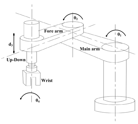
The SCARA (Selective Compliance Assembly Robot Arm) robot is a prevalent industrial manipulator and serves as a fundamental platform for research in multi-degree-of-freedom robotics [9, 10]. A typical 4-DoF SCARA robot comprises four joints: three revolute (rotational) joints and one prismatic (translational) joint, as depicted in Figure 1. Its operation is primarily within a planar workspace, making it suitable for applications such as pick-and-place operations and the precise positioning of components on a production line [11, 12].
Robot trajectory control is a critical area of study within robotics, concerned with governing the motion of a robot manipulator along a prescribed spatial path or trajectory. The primary objective is to ensure the robot achieves the desired position and orientation at specific points in time, while maintaining accuracy and stability throughout the movement. Numerous studies have addressed the problem of robot trajectory control, employing methods ranging from elementary to sophisticated ones. These approaches can be broadly classified into two categories: adaptive and non-adaptive control [13]. Non-adaptive control techniques are typically limited to basic position control and low-speed trajectory tracking, exhibiting relatively low accuracy. Conversely, adaptive control is better suited for complex robotic systems with time-varying payloads, high-speed operation, and demanding precision requirements [14-16]. This is because adaptive control offers robustness against parametric uncertainties and possesses self-tuning capabilities that accommodate system variations [17-20].
Obviously, the adaptive control is a control paradigm focused on developing flexible controllers capable of adjusting their structure or parameters to compensate for changes in the controlled system, thereby ensuring consistent performance [21]. The objective of adaptive controller design is to maintain system stability and performance despite external disturbances or unforeseen internal changes that alter the system model [22-24]. The core principle is that the controller adapts in response to system variations to maintain a desired performance level [25, 26]. Furthermore, leveraging Lyapunov stability theory enables the design of control algorithms tailored to meet diverse operational requirements under varying conditions [27]. Within a model-based framework, adaptive control algorithms are designed based on the established system model. These algorithms compensate for system uncertainties, either directly or indirectly, while respecting the inherent characteristics of the model. A continuous nonlinear controller can then be synthesized to satisfy the specified system requirements [28].
The evolution of modern control theory has facilitated the implementation of control algorithms that integrate fuzzy logic and neural networks with Model – Based Adaptive Control (MBAC). The authors proposed a hybrid control framework that synergistically combines MBAC and fuzzy logic controllers [29]. This approach capitalizes on the inherent suitability of the conventional MBAC structure for object linearization while concurrently employing a fuzzy logic controller to address the object's nonlinear dynamics. The composite input control signal is generated by the summation of the individual output signals from the fuzzy logic and MBAC components. Yu and Sun [30] presented an adaptive control architecture predicated on a fuzzy logic model. This architecture tackles a class of continuous-time nonlinear dynamical systems. The structure incorporates two distinct fuzzy logic modules: one for linearization and the other for nonlinearity compensation, with the control performance evaluated using the Lyapunov stability criterion. Alternatively, conventional MBAC can be integrated with Artificial Neural Networks (ANNs). Leveraging the principles of adaptive control, a control strategy utilizing ANNs, augmented with a disturbance observer for noise attenuation, was designed, demonstrating promising outcomes [31]. Another innovative control paradigm involves the development of an ideal dynamic model based on the Lagrangian formalism. Subsequently, the control structure employs a Deep Neural Network (DNN) to predict the real-time state of the model [32]. This new control architecture has contributed to cost reduction and enhanced dynamic compensation capabilities through feedback-driven adjustments.
This work proposes a new MBAC to a control plant class of multi-DoF robots, i.e., 4-DoF SCARA robots. Control design in step-by-step, together with theoretical analysis, will also be provided. The proposed control methodology is much simpler than several existing controllers. With better simulation results executed in MATLAB/Simulink software over other control methods, e.g., PD-G, the MBAC will be demonstrated a feasible solution for robot control in reality.
Figure 1. A typical model of a 4-DoF industrial SCARA robot
2.1 Dynamics
The robotic system comprises an n-joint manipulator, with each joint actuated to facilitate motion. During motion transitions, contact forces and sensor asynchrony can induce instability. The simultaneous operation of multiple joints introduces a range of complexities, including position and velocity deviations, estimation errors of unknown parameters, and matrix symmetry issues arising from force calculations. These forces, encompassing Coriolis and centrifugal forces, among other critical but imprecisely identified physical parameters, are incorporated within the controller's Lagrange equation.
The robot's dynamics can be represented using the Lagrange equation, which incorporates the system's physical parameters, such as mass, link moments of inertia, and inter-joint distances. Within the framework of Lagrangian mechanics, these parameters are often expressed in a linearized form. However, precise estimation of these physical parameters is not always attainable. While some parameters, such as link lengths, inter-joint distances, and the distance from a joint to the link's center of mass, can be estimated with relatively high accuracy, others remain subject to greater uncertainty.
A robot with $n$ DoFs is characterized by parameters such as mass and moment of inertia, which are expressed as coefficients of functions dependent on $q, \dot{q}$, and $\ddot{q}$. By defining each parameter, the robot dynamic equation can be formulated as follows:
$H(q) \ddot{q}+C(q, \dot{q}) \dot{q}+g(q)=Y(q, \dot{q}, \ddot{q}) \Theta=\tau$ (1)
where, the matrix $Y(q, \dot{q}, \ddot{q}) \in R^{n x r}$ is a regression matrix, while $\Theta \in R^r$ is a vector of dynamic parameters, which are unknown but must be constant.
The matrix $S(q, \dot{q})=\dot{H}(q)-2 C(q, \dot{q})$ is a skew-symmetric matrix (or an antisymmetric matrix), which satisfies the following condition:
$x^T S x=x^T(\dot{H}(q)-2 C(q, \dot{q})) x=0$ (2)
2.2 MBAC strategy
Adaptive control is a crucial field in control engineering, concerned with the design of control systems that can automatically adjust their parameters or structure to accommodate unforeseen changes in the system or operating environment. Some key characteristics of the adaptive control include:
(i) Self-tuning capability: The control system automatically modifies its parameters or structure to maintain desired performance despite variations in the system or environment.
(ii) Robustness to uncertainty: The system can handle uncertainties such as disturbances, model inaccuracies, and time-varying system parameters.
(iii) Performance maintenance: Adaptive control systems are designed to ensure stable operation and satisfy predefined performance criteria, even under changing system conditions.
This study focuses on the application of model-based adaptive control (MBAC) to a 4-DoF SCARA robot model to evaluate its efficacy and suitability for the given control problem. The system dynamics are characterized by the parameter vector Θ, as represented in the following equation [14, 18]:
$\begin{aligned} Y(q, \dot{q}, \ddot{q}) \cdot \Theta & =H(q) \cdot \ddot{q}+\left\{B_0+\frac{1}{2} \dot{H}(q)+S(q, \dot{q})\right\} \cdot \dot{q} +g(q)\end{aligned}$ (3)
During the robot's operating process, the estimated matrix $\widehat{\Theta}(0)$ of $\Theta$ should be continuously updated following a law below:
$\hat{\Theta}(t)=\hat{\Theta}(0)-\int_0^t \Gamma^{-1} \cdot Y^T\left(q_d(\tau), \dot{q}_d(\tau), \ddot{q}_d(\tau)\right) \cdot y(\tau) d t$ (4)
where, $\widehat{\Theta}(0)$ is the estimated value of $\Theta$ when $t=0$. $\Gamma$ is a $m \times m$ positive defined matrix.
Estimating the unknown parameter $\widehat{\Theta}(t)$ will be converged to a real value $\Theta$ when $t \rightarrow \infty$ and it will track the desired trajectory.
It should be obvious that the output response $y(t)$ of the system is uncertain, we can employ a real-time adaptive control law based on the established robot model:
$u=-A_1 \Delta q-B_1 z+Y\left(q, \dot{q}, q_r, \dot{q}_r\right) \hat{\Theta}$ (5)
The model-based adaptive control law and the system's parameter update law will result in trajectory convergence $\Delta q(t) \rightarrow 0$ and $\Delta \dot{q}_t \rightarrow 0$ when $t \rightarrow \infty$ in accordance with Lyapunov's stability criteria. The objective of controller design is to endow the closed-loop system, comprising both the controlled object and the controller, with desired performance characteristics. This design is predicated on Lyapunov's stability theory.
Based on the MBAC and Lyapunov's theory, the following steps should be implemented:
Step 1: Build up the control law
From Eq. (5), according to the MBAC theory, it is possible to deduce the following control law:
$M=-A_1 \Delta q-B_1 z+Y\left(q, \dot{q}, q_r, \dot{q}_r\right) \hat{\Theta}$ (6)
where,
$\Theta$ is a vector which denotes physical parameters such as mass, inertia, etc.
$\Theta=\left(I_1, m_1, \ldots, I_n, m_n\right)^T$
Let: $\left\{\begin{array}{l}q_r=\dot{q}_d-\gamma \Delta q \\ z=\dot{q}-q_r=\Delta \dot{q}+\gamma \Delta q\end{array}\right.$ with $\gamma>0$.
The parameter update rule is:
$\hat{\Theta}(t)=\hat{\Theta}(0)-\int_0^t \Gamma^{-1} Y^T\left(q(\tau), \dot{q}(\tau), q_r(\tau), \dot{q}_r(\tau)\right) z(\tau) d \tau$ (7)
and:
$\bar{Y}(q, \dot{q}, z, \dot{z}) \Theta-Y\left(q, \dot{q}, q_r, \dot{q}_r\right)+A_1 \Delta q=0$ (8)
where,
$\bar{Y}\left(q, \dot{q}, q_r, \dot{q}_r\right) \Theta=H(q) \dot{z}+\left\{B+\frac{1}{2} \dot{H}(q)+S(q, \dot{q})\right\} z$ (9)
Select a Lyapunov candidate as:
$V=\frac{1}{2} z^T H z+\frac{1}{2} \Delta q^T A_1 \Delta q+\frac{1}{2} \Delta \Theta^T \Gamma \Delta \Theta$ (10)
The Lyapunov function V in Eq. (10) is positive definite. Decomposing V into V₀ and a component dependent on the parameter update law, as shown in Eq. (11), allows for analysis of the time derivative of V.
$\begin{aligned} & \frac{d}{d t}\left\{V_0(z, \Delta q)+\frac{1}{2} \Delta \Theta^T \Gamma \Delta \Theta\right\}=z^T H \dot{z}+\frac{1}{2} z^T \dot{H} z+\Delta q^T A_1 \Delta \dot{q}+\Delta \Theta^T \Gamma \Delta \dot{\Theta}\end{aligned}$ (11)
From Eq. (1), in combination with the result $\dot{\hat{\Theta}}=\Delta \hat{\Theta}-\Gamma^{-1} Y$ deduced from Eq. (7), and by substituting Eq. (11), the following can be obtained:
$\begin{aligned} & \dot{V}=z^T[M-C \dot{q}-G+H \gamma \Delta q] +\frac{1}{2} z^T \dot{H} z+\Delta q^T A_1 \Delta q+\Delta \Theta^T Y\end{aligned}$ (12)
$\begin{aligned} \dot{V}= & z^T\left[M-C q_r-G+H \gamma \dot{q}\right]-z^T C z +\frac{1}{2} z^T \dot{H} z+\Delta q^T A_1 \Delta q+\Delta \Theta^T Y\end{aligned}$ (13)
According to the properties of system dynamics, $\dot{H}-2 C=$ 0 , substitute Eq. (4) and $z=\dot{q}-q_r=\Delta \dot{q}+\gamma \Delta q$ into Eq. (13), the following derivative can be yielded:
$\dot{V}=-z^T B_1 z-\gamma \Delta q^T A_1 \Delta q+Y \bar{\Theta}$ (14)
With $Y . \bar{\Theta}$ denotes the estimation of robot's parameters deduced from Eq. (7).
Combining Eq. (11) and Eq. (14) yields the following equation:
$\frac{d}{d t}\left\{V_0(z, \Delta q)+\frac{1}{2} \Delta \Theta^T \Gamma \Delta \Theta\right\}=-W(z, \Delta q)$ (15)
where:
$\begin{aligned} & V_0(z, \Delta q)=\frac{1}{2} z^T H(q) z+\frac{1}{2} q^T A_1 q, \\ & W_0(z, \Delta q)=z^T B z+\gamma \Delta q^T A_1 \Delta q\end{aligned}$
$\begin{aligned} W(z, \Delta q) & =\dot{z} B_1 z+\Delta \dot{q} h(z, \Delta q)-\gamma \Delta q^T H \Delta \dot{q} \\ & +\gamma \Delta q^T A_1 \Delta q+\gamma \Delta q^T\left[\left\{-\frac{1}{2} \dot{H}+S\right\} \Delta \dot{q}+h\right]\end{aligned}$ (16)
Besides,
$\begin{gathered}V(z, \Delta q) =\frac{1}{2} z^T H z+\gamma \Delta q^T H \Delta \dot{q} \\ +\frac{1}{2} \Delta q^T A_1 \Delta q+\sum_{i=1}^n \alpha b_i \Delta q_i W(z, \Delta q) \geq \Delta z^T\left\{B-\left(\bar{c}_4+\alpha \cdot \bar{c}_6\right) I\right\} z \\ +\gamma \Delta q^T\left\{A_1 D-\bar{c}_1 I\right\} \Delta q-\left(\bar{c}_3+\alpha \bar{c}_5\right)\|\Delta q\|\|z\|\end{gathered}$ (17)
With D as a diagonal matrix, when $2 a b \leq \frac{a^2}{\xi}+b^2 \xi$ with $\xi>0$ holds, Eq. (17) can be rewritten as follows:
$\begin{aligned} & W(z, \Delta q) \geq \frac{1}{2}\left\{z^T B z+\gamma \Delta q^T A_1 D \Delta q\right\} \\ & +\frac{1}{2} z^T\left[B-\left\{2 \bar{c}_4+\alpha\left(2\left(\bar{c}_2+\bar{c}_6\right)+\bar{c}_5\right)+\bar{c}_3 \sqrt{\frac{\gamma}{\alpha}}\right\} I\right] z \\ & +\frac{\alpha}{2} \Delta q^T\left\{A_1 D-\left(2 \bar{c}_1+\bar{c}_5+\bar{c}_3 \sqrt{\gamma \alpha}\right) I\right\} \Delta q\end{aligned}$ (18)
where, $\gamma$ is a positive arbitrary number, and the function $V$ can be rewritten as:
$\begin{aligned} V(\Delta q, z) & \geq \frac{1}{4} z^T H(q) z+\frac{1}{2} \Delta q^T A_1 \Delta q +\sum_{i=1}^n \alpha\left\{b_i c_i-\alpha \gamma_M\right\} s_i^2\left(\Delta q_i\right)\end{aligned}$ (19)
To summarise, with $\alpha>0$, two matrices $\mathrm{A}_1$ and $\mathrm{B}_1$ are chosen to satisfy the following condition:
$B_0 \geq \alpha \gamma_M C^{-1}$ (20)
$\begin{gathered}A_1 \geq\left(2 \bar{c}_1+\bar{c}_5+\frac{\bar{c}_3}{\sqrt{\alpha \gamma}}\right) D^{-1} \\ B_1 \geq\left\{2 \bar{c}_4+\alpha\left(2\left(\bar{c}_2+\bar{c}_6\right)+\bar{c}_5\right)+\bar{c}_3 \sqrt{\frac{\gamma}{\alpha}}\right\} I\end{gathered}$ (21)
When C is a diagonal matrix with elements cᵢ and γ are given by appropriate constants.
With B = B₀ + B₁, inequalities Eq. (20) and Eq. (21) imply the positive definiteness of V and W with respect to the variables z. From this, it is reasonable to yield Eq. (22):
$\begin{aligned} & \int_0^t\{\Delta \dot{q}+\gamma(\Delta q)\}^T \Delta v d \tau \\ & =V(\Delta q(t), z(t))-V(\Delta q(0), z(0)) \\ & +\int_0^t W(\Delta q(\tau), z(\tau)) d \tau \\ & \geq-V(\Delta q(0), z(0))=-\gamma_0^2\end{aligned}$ (22)
With factors $\bar{c}_i(i=1, \ldots, 6)$ are chosen to be positive and dependent on the desired values. Combining the conditions from Eq. (20) and Eq. (21), with $W(z, \Delta q)=W_0(z, \Delta q)+$ $W_1(z, \Delta q)$.
So,
$\begin{aligned} & W_1(z, \Delta q) \\ & \geq \frac{1}{2} z^T\left[B-\left\{2 \bar{c}_4+\alpha\left(2\left(\bar{c}_2+\bar{c}_6\right)+\bar{c}_5\right)+\bar{c}_3 \sqrt{\frac{\gamma}{\alpha}}\right\} I\right] z \\ & +\frac{\alpha}{2} \Delta q^T\left\{A_1 D-\left(2 \bar{c}_1+\bar{c}_5+\bar{c}_3 \sqrt{\gamma \alpha}\right) I\right\} \Delta q\end{aligned}$ (23)
It is clear that the right site of Eq. (23) is always positive, and the function $W(z, \Delta q)$ is a positive matrix, then $W(z, \Delta q)<0$.
Based on the Lyapunov stability criterion, the MBAC rule mentioned above will treat the closed-loop control to be stable.
Some of advantages of this approach include:
(i) High accuracy without requiring precise knowledge of the robot's parameters.
(ii) Compensation for inter-joint nonlinearities.
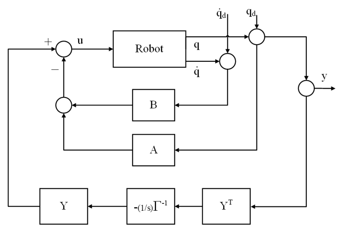
This control methodology may have slight disadvantages. High computational cost, as the controller design is predicated on the robot's dynamics and necessitates direct parameter identification and updating. Besides, the selection of external parameters for the identification matrix significantly influences both system stability and transient response. The MBAC control law block diagram is presented in Figure 2.
Figure 2. A schematic diagram of the MBAC algorithm to control a 4-DoF industrial SCARA robot
It is clear simulation is an initialization step which is highly significant to examine the effectiveness of a control strategy. Also, applying an efficient simulation tool plays a crucial role to verify precisely controlling the performance of the systems under study. This work employs MATLAB/Simulink for such a simulation process. The capability to construct visual models via Simulink's graphical user interface facilitates the simulation of complex systems by engineers, thereby enabling the evaluation and optimization of control parameters prior to physical implementation. Therefore, simulation with MATLAB/Simulink contributes to the reduction of time and cost, while concurrently enhancing the reliability and efficacy of control systems.
To execute the simulation process, let us consider the parameters of a 4-DoF robot given in Table 1.
Table 1. Simulation parameters for the 4-DoF robot model
|
No. |
Parameter |
Value |
Unit |
|
1 |
Main arm (lengh) |
0.25 |
[m] |
|
2 |
Main movement (θ1) |
200 |
[degree] |
|
3 |
Fore arm (lengh) |
0.15 |
[m] |
|
4 |
Fore arm movement (θ2) |
250 |
[degree] |
|
5 |
Arm up-down (d3) (lengh) |
0.75 |
[m] |
|
6 |
Arm up-down (d3) (lengh) |
0.75 |
[m] |
|
7 |
Wrist rotation (θ4) |
450 |
[degree] |
|
8 |
Moment of inertia of the 1st joint (J1) |
0.098 |
[kg.m2] |
|
9 |
Moment of inertia of the 2nd joint (J2) |
0.0115 |
[kg.m2] |
|
10 |
Moment of inertia of the 4th joint (J4) |
0.005 |
[kg.m2] |
|
11 |
Mass of the 1st joint (m1) |
1.9 |
[kg] |
|
12 |
Mass of the 2nd joint (m2) |
0.93 |
[kg] |
|
13 |
Mass of the 4th joint (m4) |
0.3 |
[kg] |
To emphasize the dominant performance of the proposed MBAC, the robotic system also executes the simulation with a PD-G (Proportional-Derivative plus Gravity compensation) control algorithm [33-35].
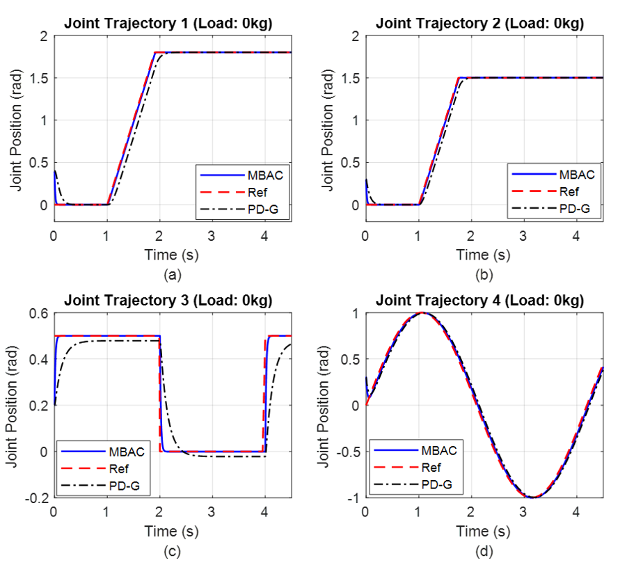
Figure 3. Simulation results for all joints in case 1 with no load
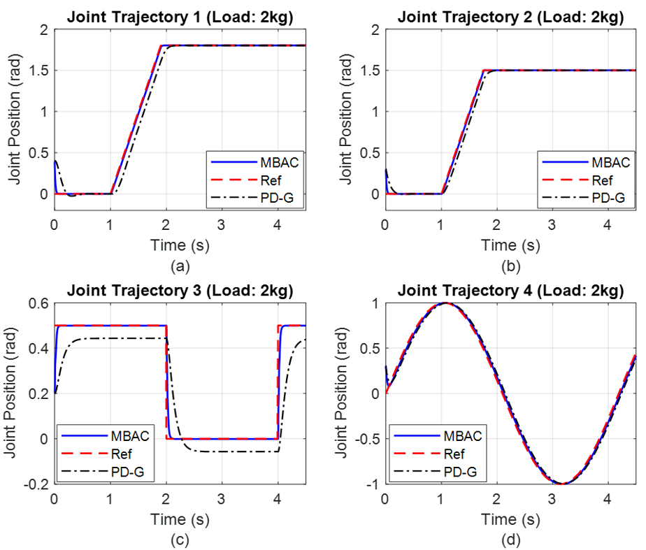
Figure 4. Simulation results for all joints in case 1 with load 2 kg
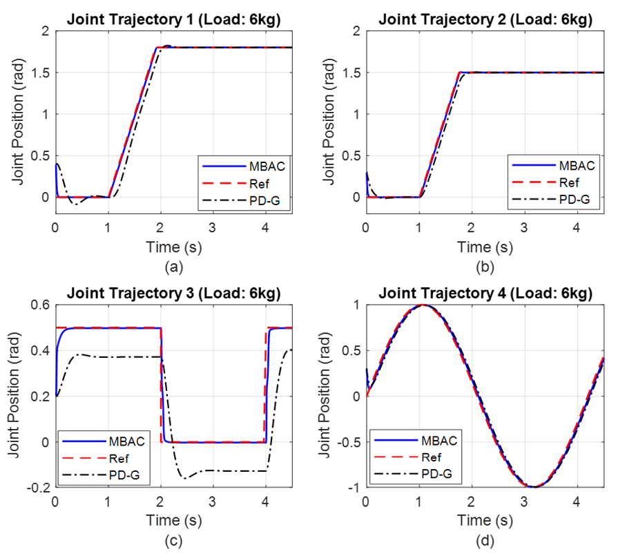
Figure 5. Simulation results for all joints in case 1 with load 6 kg
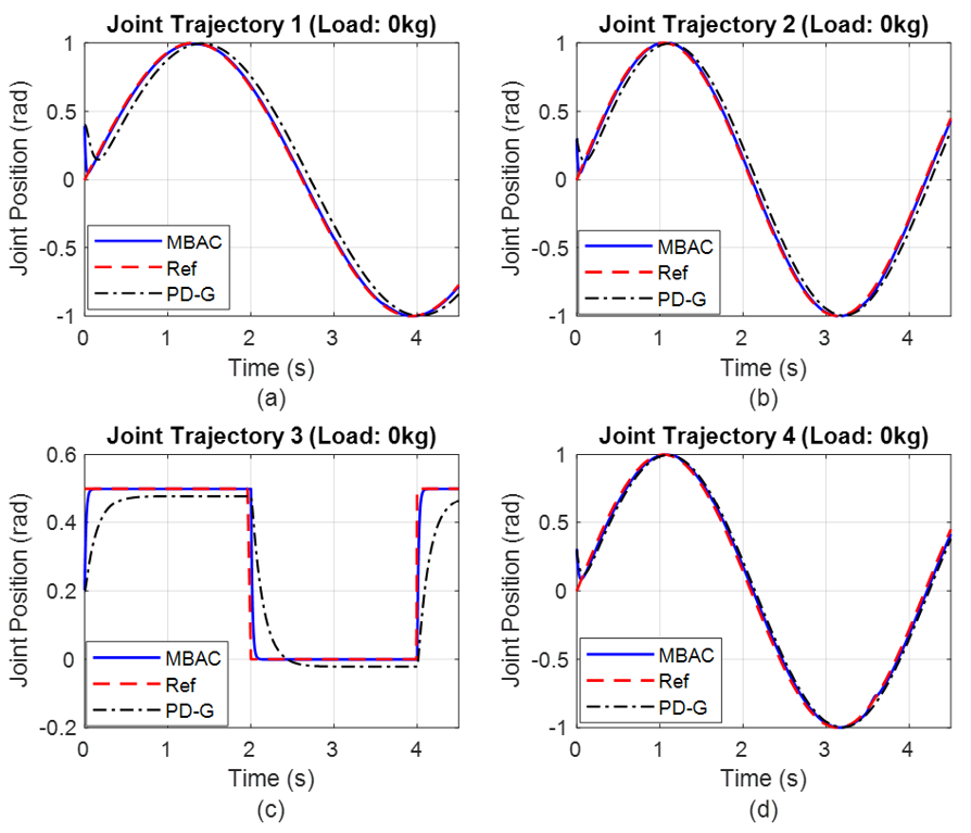
Figure 6. Simulation results for all joints in case 2 with no load
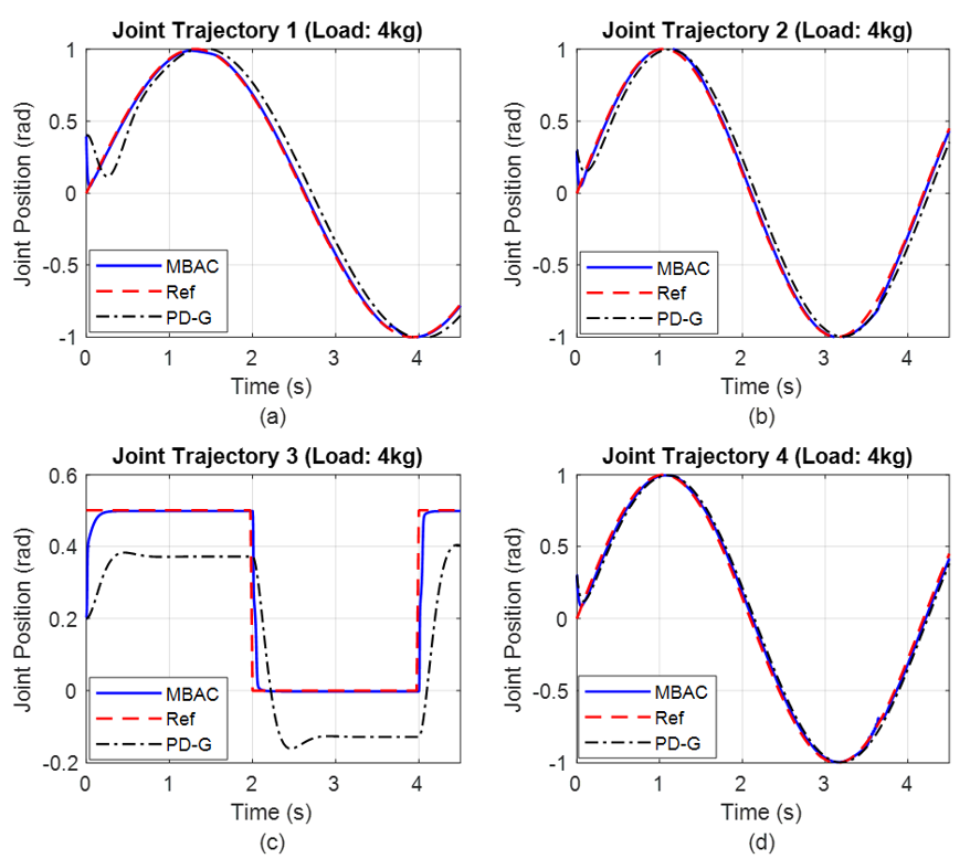
Figure 7. Simulation results for all joints in case 2 with load 4 kg
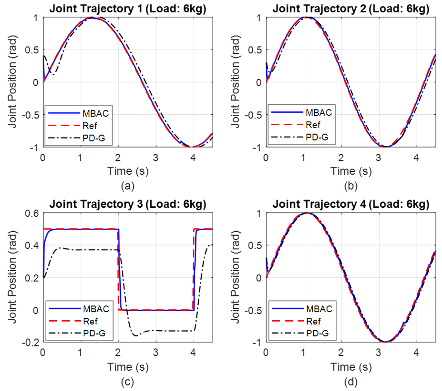
Figure 8. Simulation results for all joints in case 2 with load 6 kg
This study investigates two distinct simulation scenarios, each employing varying payloads, specifically 0 kg, 2 kg, 4 kg, and 6 kg, to assess system performance under load variations ranging from no-load to a maximum of 6 kg.
(i) Case 1: The desired trajectories for joints 1 and 2 are presented in Figures 3-5 (a) and (b), respectively. The corresponding trajectory tracking responses for joints 3 and 4 are illustrated in Figures 3-5 (c) and (d). Within these figures, the desired trajectory is denoted by a red dashed line, the PD-G controller's response by a black dashed-dot line, and the proposed MBAC controller's response by a solid blue line.
(ii) Case 2: Sinusoidal desired trajectories for joints 1 and 2 are depicted in Figures 6-8 (a) and (b). Similarly, the tracking responses for joints 3 and 4 are shown in Figures 6-8 (c) and (d).
The simulation results reveal a diverse spectrum of trajectory tracking responses, clearly demonstrating the superior control performance of the MBAC method compared to the PD-G approach. Across all simulation cases, the MBAC controller exhibited responses characterized by minimal overshoot, short settling times, rapid rise times, and negligible steady-state errors. Conversely, the PD-G controller displayed significant overshoot and suboptimal performance across other metrics, including substantial steady-state errors. Notably, the PD-G controller's performance is highly susceptible to payload variations, with significant degradation observed under both no-load and maximum-load conditions. In contrast, the proposed MBAC controller demonstrated robust performance, largely unaffected by payload changes, thereby underscoring a key advantage of the proposed control strategy.
Some of the other comments on the MBAC algorithm are as follows:
The MBAC law fulfills the accuracy requirements and ensures timely response, thus rendering it a suitable control law for the SCARA robot manipulator.
Simulation results demonstrate that the 4-DoF robotic arm, under model-based adaptive control, accurately tracks predefined trajectories. The steady-state and dynamic angular displacement errors are minimal. Under varying load conditions, while angular and velocity errors do exhibit changes, they remain within a narrow tolerance. Comparative simulations between non-adaptive (PD-G) and model-based adaptive control (MBAC) reveal that MBAC outperforms PD-G. System performance, in terms of quality and settling time, is assessed through simulations involving variations in both the desired trajectory and the robot's load during motion. The findings indicate that with MBAC, the system exhibits rapid response while maintaining precise trajectory tracking with minimal deviation.
The MBAC, even obtaining a lot of dominant performances, still has limitations as presented below:
Future research will focus on evaluating the MBAC algorithm in conjunction with intelligent techniques, such as fuzzy logic and neural networks. Furthermore, robotic arms with higher degrees of freedom (e.g., 6-DOF) may serve as target platforms for the proposed control algorithm. Given the expanding range of industrial applications, the integration of AI-powered recognition and quality classification functionalities into industrial robotic arms warrants consideration in future research endeavors.
[1] Hazem, Z.B., Ince, R., Dilibal, S. (2022). Joint control implementation of 4-DOF robotic arm using robot operating system. In 2022 International Conference on Theoretical and Applied Computer Science and Engineering (ICTASCE), Ankara, Turkey, pp. 72-77. https://doi.org/10.1109/ICTACSE50438.2022.10009733
[2] Ting, H.Z., Hairi, M., Zaman, M., Ibrahim, M., Moubark, A. (2021). Kinematic analysis for trajectory planning of open-source 4-DoF robot arm. International Journal of Advanced Computer Science and Applications, 12(6): 769-777. https://doi.org/10.14569/IJACSA.2021.0120690
[3] Dewi, T., Nurmaini, S., Risma, P., Oktarina, Y., Roriz, M. (2020). Inverse kinematic analysis of 4 DOF pick and place arm robot manipulator using fuzzy logic controller. International Journal of Electrical & Computer Engineering (2088-8708), 10(2): 1376-1386. https://doi.org/10.11591/ijece.v10i2.pp1376-1386
[4] Benosman, M. (2016). Learning-based adaptive control: An extremum seeking approach–theory and applications. Butterworth-Heinemann.
[5] Raja, R.I., Kareem, I.S., Abdul-Lateef, W.E. (2024). Kinematic analysis model of 4-DOF robotic arm. In AIP Conference Proceedings, Baghdad, Iraq, 030001. https://doi.org/10.1063/5.0206140
[6] Zhang, D., Wei, B. (2017). A review on model reference adaptive control of robotic manipulators. Annual Reviews in Control, 43: 188-198. https://doi.org/10.1016/j.arcontrol.2017.02.002
[7] Ventura–Hinostroza, H., Rojas–Moreno, A. (2019). Real–time model reference adaptive control of a 3DOF robot arm. In 2019 IEEE XXVI International Conference on Electronics, Electrical Engineering and Computing (INTERCON), Lima, Peru, pp. 1-4. https://doi.org/10.1109/INTERCON.2019.8853622
[8] Li, Y., Wang, L. (2022). Kinematic model and redundant space analysis of 4-dof redundant robot. Mathematics, 10(4): 574. https://doi.org/10.3390/math10040574
[9] Das, M.T., Dulger, L.C. (2010). Control of a SCARA robot: PSO-PID approach. Control and Intelligent Systems, 38(1): 24-31.
[10] Er, M.J., Liew, K.C. (1997). Control of adept one SCARA robot using neural networks. IEEE Transactions on Industrial Electronics, 44(6): 762-768. https://doi.org/10.1109/41.649936
[11] Ibrahim, B.S.K.K., Zargoun, A.M. (2014). Modelling and control of SCARA manipulator. Procedia Computer Science, 42: 106-113. https://doi.org/10.1016/j.procs.2014.11.040
[12] Urrea, C., Cortés, J., Pascal, J. (2016). Design, construction and control of a SCARA manipulator with 6 degrees of freedom. Journal of Applied Research and Technology, 14(6): 396-404. https://doi.org/10.1016/j.jart.2016.09.005
[13] Meng, Q.H.M. (1995). Comparison study of model-based and non-model-based robot controllers. In 1995 IEEE International Conference on Systems, Man and Cybernetics. Intelligent Systems for the 21st Century, Vancouver, BC, Canada, pp. 61-66. https://doi.org/10.1109/ICSMC.1995.537734
[14] Arimoto, S., Liu, Y.H., Naniwa, T. (1993). Model-based adaptive hybrid control for geometrically constrained robots. In 1993 Proceedings IEEE International Conference on Robotics and Automation, Atlanta, GA, USA, pp. 618-623. https://doi.org/10.1109/ROBOT.1993.292047
[15] Akella, P., Parra-Vega, V., Arimoto, S., Tanie, K. (1994). Discontinuous model-based adaptive control for robots executing free and constrained tasks. In Proceedings of the 1994 IEEE International Conference on Robotics and Automation, San Diego, CA, USA, pp. 3000-3007. https://doi.org/10.1109/ROBOT.1994.351108
[16] Pandian, S.R., Hanmandlu, M. (1993). Adaptive generalized model-based control of robot manipulators. International Journal of Control, 58(4): 835-852. https://doi.org/10.1080/00207179308923031
[17] Ciliz, M.K., Narendra, K.S. (1994). Multiple model based adaptive control of robotic manipulators. In Proceedings of 1994 33rd IEEE Conference on Decision and Control, Lake Buena Vista, FL, USA, pp. 1305-1310. https://doi.org/10.1109/CDC.1994.411141
[18] Naniwa, T., Arimoto, S., Vega, V.P. (1994). A model-based adaptive control scheme for coordinated control of multiple manipulators. In Proceedings of IEEE/RSJ International Conference on Intelligent Robots and Systems (IROS'94), Munich, Germany, pp. 695-702. https://doi.org/10.1109/IROS.1994.407357
[19] Franco, E., Casanovas, A.G., y Baena, F.R., Astolfi, A. (2019). Model based adaptive control for a soft robotic manipulator. In 2019 IEEE 58th Conference on Decision and Control (CDC), Nice, France, pp. 1019-1024. https://doi.org/10.1109/CDC40024.2019.9029449
[20] Benosman, M. (2018). Model-based vs data-driven adaptive control: An overview. International Journal of Adaptive Control and Signal Processing, 32(5): 753-776. https://doi.org/10.1002/acs.2862
[21] Silvia, F.R., Stengel, F. (2004). Model-based adaptive critic designs. Handbook of Learning and Approximate Dynamic Programming.
[22] Hassanein, O., Anavatti, S.G., Shim, H., Ray, T. (2016). Model-based adaptive control system for autonomous underwater vehicles. Ocean Engineering, 127: 58-69. https://doi.org/10.1016/j.oceaneng.2016.09.034
[23] Portillo, R., Vazquez, S., Leon, J.I., Prats, M.M., Franquelo, L.G. (2012). Model based adaptive direct power control for three-level NPC converters. IEEE Transactions on Industrial Informatics, 9(2): 1148-1157. https://doi.org/10.1109/TII.2012.2209667
[24] Barber, R., Rosa, D.R., Flores-Caballero, A., Garrido, S. (2023). Deployment of model-based-design-adaptive controllers for monitoring and control mechatronic devices. Applied Sciences, 13(22): 12432. https://doi.org/10.3390/app132212432
[25] Scherler, S., Liu-Henke, X. (2018). Model-based design of a multi-functional HiL test bench for investigations on a Range Extended Vehicle. In 2018 IEEE International Systems Engineering Symposium (ISSE), Rome, Italy, pp. 1-7. https://doi.org/10.1109/SysEng.2018.8544400
[26] Chen, Z., Niu, B., Zhao, X., Zhang, L., Xu, N. (2021). Model-based adaptive event-triggered control of nonlinear continuous-time systems. Applied Mathematics and Computation, 408: 126330. https://doi.org/10.1016/j.amc.2021.126330
[27] Yu, H., Hao, F. (2015). Adaptive model-based event-triggered control for linear systems. In 2015 34th Chinese Control Conference (CCC), Hangzhou, China, pp. 6630-6635. https://doi.org/10.1109/ChiCC.2015.7260684
[28] Della Santina, C., Katzschmann, R.K., Bicchi, A., Rus, D. (2020). Model-based dynamic feedback control of a planar soft robot: trajectory tracking and interaction with the environment. The International Journal of Robotics Research, 39(4): 490-513. https://doi.org/10.1177/0278364919897292
[29] Prakash, R., Anita, R. (2012). Modeling and simulation of fuzzy logic controller-based model reference adaptive controller. International Journal of Innovative Computing, Information and Control, 8(4): 2533-2550.
[30] Yu, W.S., Sun, C.J. (2001). Fuzzy model based adaptive control for a class of nonlinear systems. IEEE Transactions on Fuzzy Systems, 9(3): 413-425. https://doi.org/10.1109/91.928738
[31] Li, T., Zhang, G., Zhang, T., Pan, J. (2024). Adaptive neural network tracking control of robotic manipulators based on disturbance observer. Processes, 12(3): 499. https://doi.org/10.3390/pr12030499
[32] Guo, D., Xie, Z., Sun, X., Zhang, S. (2023). Dynamic modeling and model-based control with neural network-based compensation of a five degrees-of-freedom parallel mechanism. Machines, 11(2): 195. https://doi.org/10.3390/machines11020195
[33] Euldji, R., Batel, N., Rebhi, R., Lorenzini, G., Jarasthitikulchai, N., Menni, Y., Sudsutad, W. (2022). Optimal design and performance comparison of a combined ANFIS-PID with back stepping technique, using various meta-heuristic algorithms to solve wheeled mobile robot trajectory tracking problem. Journal Européen des Systèmes Automatisés, 55(3): 281-298. https://doi.org/10.18280/jesa.550301
[34] Perrusquía, A., Flores-Campos, J.A., Torres-San-Miguel, C.R. (2020). A novel tuning method of PD with gravity compensation controller for robot manipulators. IEEE Access, 8: 114773-114783. https://doi.org/10.1109/ACCESS.2020.3003842
[35] Xu, T., Feng, Y., Wu, S., Chen, Z., Wu, K., Li, J., Zhan, B. (2023). Study on adaptive PD control of dexterous arm based on gravity compensation. In 2023 5th International Symposium on Robotics & Intelligent Manufacturing Technology (ISRIMT), Changzhou, China, pp. 213-220. https://doi.org/10.1109/ISRIMT59937.2023.10428338