Habeeb J. Nekad*![]() | Diyah Kammel Shary
| Diyah Kammel Shary![]() | Mazin Abdulelah Alawan
| Mazin Abdulelah Alawan![]()
© 2024 The authors. This article is published by IIETA and is licensed under the CC BY 4.0 license (http://creativecommons.org/licenses/by/4.0/).
OPEN ACCESS
Due to a non-linearity characteristic for linear synchronous reluctance motor (LSRM) magnetic circuit, which generate significant overshoots and oscillations in the device's movement. Two different kinds of controllers are used to verify the position of the motor: a traditional Proportional Integral (PI) controller and a modified camel traveling algorithm (MCTA) with PI controller. In the first the dynamic model of LSRM is presented in d-q reference frame and simulated using MATLAB Simulink program (MATLAB 2022a) with using actual position as a feedback signal. The motor position is tested in three different reference position trajectories: trapezoidal reference position trajectory, linear reference position trajectory, and non-linear reference position trajectory. The outcomes demonstrate how well the employed controllers improved the position and velocity responses of the motor performance under various reference position trajectories.
linear synchronous reluctance motor, position control, velocity control, PI controller, modified camel traveling algorithm
Direct-drive linear systems offer several benefits over typical (indirect) drive rotary motor systems. There is no need for a mechanical transmission when applying the electromechanical force from a linear motor straight to the pay load. Moreover, the linear motor drive systems have less friction, minimal backlash, need no mechanical maintenance, and have a longer lifespan [1-7].
Linear electric motors are electromechanical devices that generate motion in a straight line without utilizing a mechanism to convert rotational motion to linear motion. Linear motors have a virtually identical history as rotary motors. Due to its advantages over other types of linear motors, the use of linear synchronous reluctance motors (LSRM) for a variety of applications continues to grow. Their key benefits include cheap reaction rail components, the absence of substantial heat sources during reaction rail operation, and the fact that only the reaction rail portion opposite the armature is exposed to the magnetic field when the reaction rail is in use [8-15].
Since the magnetic circuit of the LSRM exhibits nonlinear properties, the movement of the device exhibits large overshoots and oscillations. Because of the LSRM's nonlinear magnetic circuit, a typical PI controller is inadequate. Also, several high-precision control and observation techniques were created over the last ten years. In 2011, for high-precision applications, Pupadubsin et al. [16] created an adaptive sliding-mode position control of a coupled-phase linear variable reluctance (LVR) motor. Due to its simple structure, compact size, low cost, and lack of a permanent magnet, LVR motor can be seen as a good contender for high-performance linear motion applications. The sliding-mode adaptive position controller is taken into consideration due to its straightforward construction and resistance to ambiguous perturbations and outside disturbances. The comparative experimental findings unmistakably demonstrate that the suggested controller is efficient in decreasing chattering while being appropriate for regulating the LVR motor system for high-accuracy applications [16]. In 2019, to regulate the mover position of a permanent magnet linear synchronous motor (PMLSM) system, Chen et al. [17] developed an adaptive fuzzy fractional-order sliding-mode control (AFFSMC) technique. A novel fractional-integral sliding surface is used to build a fractional-order sliding-mode control (FSMC). In a further development of the AFFSMC, an uncertainty observer is created to monitor uncertainties, and an adaptive fuzzy reaching regulator is created to simultaneously account for observational errors and reduce chattering. Experiments show that the suggested AFFSMC system provides the exact tracking response for the PMLSM drive system and the robust control performance against parameter fluctuations and external disturbances [17]. In 2019, Wang et al. [18] proposed a magnetic sensor-based embedded position detecting approach for (PMLSM). To demonstrate the viability, Tunnel magneto resistance (TMR) sensors with a single axis sensitive direction are used as the sensing component. The PMLSM magnet is included in the suggested system as a sensor component, in contrast to the conventional magnetic displacement sensor bundled with a magnetic grid. TMR sensors spaced half the pole pitch apart and stimulated with alternating voltages are used to detect the shifting magnetic field as the PMLSM moves. The suggested technology is attractive from an industrial standpoint because it is non-contact, high resolution, and miniaturized [18]. In 2022, Shi and Lan [19] presented an improved predictive position control (IPPC) approach for linear synchronous motors (LSM) according to the disturbance observer (DOB) to improve tracking precision and robustness to parameter mismatches and load disturbances. To improve tracking accuracy, a soft constraint is built for the cost function that includes the gap between projected tracking errors and their exponential convergence trajectory. The Lyapunov stability theory and Bellman's principle of optimality are used to examine stability of the control system. The experimental results show that the control method is effective [19].
In this paper LSRM's three-phase dynamic model is demonstrated and simulated using the MATLAB Simulink application. Moreover, a conventional proportional integral (PI) controller and a modified camel traveling algorithm (MCTA) with PI controller are both employed to validate the position of the LSRM. Several reference position trajectories are used to assess the motor position. The results demonstrate the motor's capacity for quick responses using reference position trajectories. The camel algorithm also decreases position inaccuracy and enhances the motor's response to position and velocity.
2.1 Dynamic model of synchronous linear reluctance motor
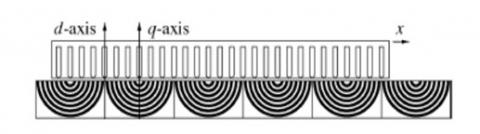
The linear synchronous reluctance motor's (LSRM) schematic diagram is shown in Figure 1. Due to the low ratio of d-axis permeance to q-axis permeance, the thrust of such a motor is minimal. The primary of this motor is short and moving (mover). The three-phase dynamic model of LSRM is given according to the following equations [20, 21]:
$\left[\begin{array}{l}V_a \\ V_b \\ V_c\end{array}\right]=\left[\begin{array}{lll}R & 0 & 0 \\ 0 & R & 0 \\ 0 & 0 & R\end{array}\right]\left[\begin{array}{l}i_a \\ i_b \\ i_c\end{array}\right]+\frac{d}{d t}\left[\begin{array}{l}\lambda_a \\ \lambda_b \\ \lambda_c\end{array}\right]$ (1)
$\lambda=L i$ (2)
$F_e=\frac{1}{2} i_{a b c}^T \frac{\partial L_{a b c}}{\partial x} i_{a b c}$ (3)
where, Va, Vb, Vc are the three-phase voltages of the primary (V), ia, ib, ic are the primary's three-phase currents (A), R is the primary phase resistance (W), la, lb, lc are the flux linkages of the primary (Wb.T), L is the inductance (H), Fe is the electromagnetic thrust of the motor (N), x is the primary's position (m).
Figure 1. Schematic diagram of LSRM
Two-axis model of LRM can be used to simplify the solution of challenging equations or to refer all variables to a common reference frame. Two-axis linear motor dynamic models are normally used for the control synthesis. The direct axis "d" and the quadrature axis "q" of a two-axis LRM model are defined by axis of the minimum and the maximum magnetic reluctances. The two-axis dq model of a LRM can be derived from the three-phase model by using the transformation matrix "T" to transfer the voltage and current vectors from abc reference frame to dq reference frame. The three-phase variables in the above equations can be expressed in d-q reference frame by using the following transformation:
$\left.\begin{array}{rl}V_{d q 0} & =T V_{a b c} \\ i_{d q 0} & =T i_{a b c} \\ \lambda_{d q 0} & =T \lambda_{a b c}\end{array}\right\}$ (4)
where, Vdq0, idq0, and ldq0, are d-q corresponding reference frame voltages, currents, and flux linkages. T denotes the transformation matrix which can be given as [20, 21]:
$T=\sqrt{\frac{2}{3}}\left[\begin{array}{ccc}\cos \left(\frac{\pi}{\tau_p} x\right) & \cos \left(\frac{\pi}{\tau_p} x-\frac{2 \pi}{3}\right) & \cos \left(\frac{\pi}{\tau_p} x+\frac{2 \pi}{3}\right) \\ -\sin \left(\frac{\pi}{\tau_p} x\right) & -\sin \left(\frac{\pi}{\tau_p} x-\frac{2 \pi}{3}\right) & -\sin \left(\frac{\pi}{\tau_p} x+\frac{2 \pi}{3}\right) \\ \frac{1}{\sqrt{2}} & \frac{1}{\sqrt{2}} & \frac{1}{\sqrt{2}}\end{array}\right]$ (5)
$T^{-1}=\sqrt{\frac{2}{3}}\left[\begin{array}{ccc}\cos \left(\frac{\pi}{\tau_p} x\right) & -\sin \left(\frac{\pi}{\tau_p} x\right) & \frac{1}{\sqrt{2}} \\ \cos \left(\frac{\pi}{\tau_p} x-\frac{2 \pi}{3}\right) & -\sin \left(\frac{\pi}{\tau_p} x-\frac{2 \pi}{3}\right) & \frac{1}{\sqrt{2}} \\ \cos \left(\frac{\pi}{\tau_p} x+\frac{2 \pi}{3}\right) & -\sin \left(\frac{\pi}{\tau_p} x+\frac{2 \pi}{3}\right) & \frac{1}{\sqrt{2}}\end{array}\right]$ (6)
where, $\tau_p$ is the primary pole pitch. Due to the star connection, the current's zero component i0 equals zero. So that the voltage equation in d-q reference frame can be written as:
$\begin{gathered}{\left[\begin{array}{l}V_d \\ V_q\end{array}\right]=\left[\begin{array}{ll}R & 0 \\ 0 & R\end{array}\right]\left[\begin{array}{l}i_d \\ i_q\end{array}\right]+\left[\begin{array}{cc}L_d & 0 \\ 0 & L_q\end{array}\right] \frac{d}{d t}\left[\begin{array}{l}i_d \\ i_q\end{array}\right]+} \\ \frac{\pi}{\tau_p}\left[\begin{array}{cc}0 & -L_q \\ L_d & 0\end{array}\right]\left[\begin{array}{l}i_d \\ i_q\end{array}\right]\end{gathered}$ (7)
where, Vd, Vq voltages for the d-q reference frame (V), id, iq currents in the d-q reference frame (A), Ld is the direct axis inductance (H), Lq is the quadrature axis inductance (H).
The electromagnetic thrust of LRM and the linear motor mechanical equations are given as:
$F_e=\frac{\pi}{\tau_p}\left(L_d-L_q\right) i_d i_q$ (8)
$m \frac{d^2 x}{d t^2}=F_e-F_l-b \frac{d x}{d t}$ (9)
$v=\frac{d x}{d t}$ (10)
where, Fl is the load force (N), m is the mass of the primary (kg), b is the friction coefficient (Ns/m), v is the linear velocity of the mover (m/sec.).
2.2 LSRM Simulink model
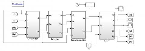
The overall block diagram of LSRM MATLAB Simulink to evaluate its performance is provided in Figure 2, which is comprised of four blocks (controller block, inverter block, transformation block, and internal construction block of the motor).
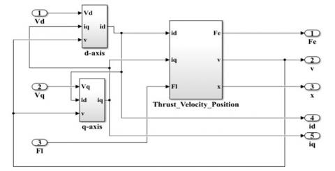
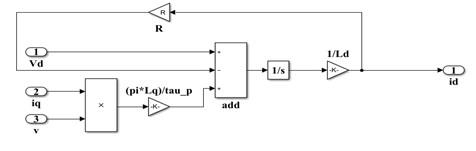
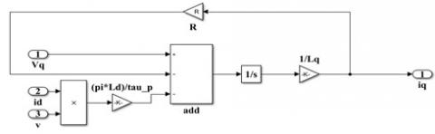
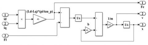
The internal building block of the LSRM is depicted in Figure 3 according to Eq. (7) through Eq. (10). It is obvious that the d-axis block, q-axis block, and another block used to calculate the thrust force, velocity, and position of this motor are the building blocks used to construct Figures 3-6 respectively, show the specifics of these blocks.
Figure 2. Overall block diagram of LSRM
Figure 3. Internal construction diagram of LSRM
Figure 4. D-axis block
Figure 5. Q-axis block
Figure 6. Thrust force, velocity, and position block
2.3 PI controller
The conventional PI can be considered as a foundation stone algorithm in the theory of control. Many systems use this control algorithm because it is smooth and precise. One method for adjusting these values is by trial and error. The control decision of the regulation is set mathematically according to [22-27]:
$u(t)=K_p e(t)+K_i \int e(t) d t$ (11)
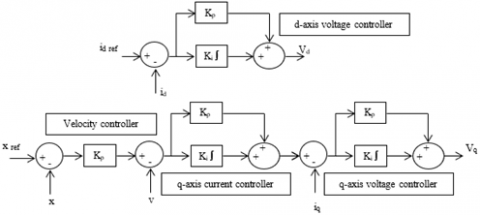
where, u(t) is the output signal, e(t) is the error signal, Kp is the proportional constant, and Ki is the integral constant. The controller block, which represents the motor's PI controller operation, is given in Figure 7. To determine the voltages for the d-q reference frame, this block is made comprised of the d-axis controller and the q-axis controller.
Figure 7. LSRM PI controller block
2.4 Modified camel traveling algorithm
It is one of the algorithms used to optimize parameter values. This technique, which is based on the way a camel behaves when traveling and how it locates food, produces superb results when modifying the PI parameters. The camel traveling algorithm (CTA) algorithm, which consists of multi-loop nesting and multiple parameter selection, has a complicated structure that adversely impacts the memory capacity and processing speed. Nevertheless, the simplified structure of the MCTA greatly accelerated its convergence and computing time.
MCTA is faster than the original CTA and other optimization methods [28].
The following points may be used to summarize the general structure of the camel algorithm:
The structure of the modified camel algorithm MCTA that mimics camels travelling behavior is easy because there are less setting parameters than in the old one. In order to implement the MCTA, it is suggested that N camels (the Camel Caravan) move through a (D)-dimensional environment of camels, and it is shown that the flow is $\left(x^{i, i t r}\right)$ which represents the location of the camel (i) at time iteration (itr) [28, 29].
$\begin{aligned} & x^{i, i t r}=\left\{x_1^{i, i t r}, x_2^{i, i t r}, \ldots, x_D^{i, i t r}\right\} \\ & i=1,2, \ldots \ldots, N\end{aligned}$ (12)
where, itr is iteration, $i t r=1,2, \ldots \ldots, i t r_{\max }$, the starting position is determined by using the following equation in the beginning (itr=0), when the camels are dispersed around the desert and are scavenging at random for food and water:
$x_d^{i t r}=\left(x_{\max }-x_{\min }\right) R+x_{\min }$ (13)
where, $R \in[0,1], d=1,2, \ldots ., D, x_d^{i t r}:$ Location of a camel, $x_{\max }$: Maximum location of a camel, and $x_{\min }$: Minimum location of a camel.
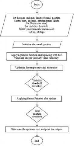
Figure 8. Flow chart of MCTA
The process as a whole is significantly influenced by the environment's temperature (T), hence the temperature for the camel throughout the iteration (iter) may be used to indicate this as shown below:
$T_d^{i t r}=\left(T_{\max }-T_{\min }\right)$ Rand $+T_{\min }$ (14)
where, Rand $\in[0,1], T_d^{i t r}$ represents the temperature and $T_{\min }$ and $T_{\max }$ represent the minimum and maximum amount of temperature, respectively. The relationship between temperature and camel endurance $\left(E_d^{i t r}\right)$ at the time iteration may be seen as follows:
$E_d^{i t r}=1-\frac{\left(T_d^{i t r}-T_{\min }\right)}{\left(T_{\max }-T_{\min }\right)}$ (15)
The visibility (v) option, which has a random value between 0 and 1, is used to update the camel's position. Dunes may impede some camels' vision, preventing them from altering their course toward the water and food source located by a specific camel. Additionally, there are two ways to update each camel's location. MCTA flowchart is shown in Figure 8. - If v < visibility threshold, the update location follows Eq. (13). - If v > visibility threshold, the update location equation is:
$x_d^{i t r}=x_d^{i t r-1}+\left(x_d^{b e s t}-x_d^{i, i t r-1}\right) E_d^{i, i t r}$ (16)
To ascertain whether the new location of $x_d^{i t r}$ is superior to the previous best location, the fitness function is applied to the new location of $x_d^{i t r}$. If this value outperforms the previous best value, the output is at its best. This output shows the optimal gain values, where $x_1^{i t r}$ stands for $K_p$ and $x_2^{i t r}$ for $K_i$.
The d-q model of LSRM is verified by MATLAB software. Its parameters are listed in Table 1. This motor is tested under different conditions to evaluate the position response. Three types of reference position trajectories are used:
1) Trapezoidal reference position trajectory,
2) Linear reference position trajectory,
3) Non-linear reference position trajectory according the following equation [21]:
$x_{r e f}=\frac{0.75}{2 \pi}[2 \pi t-\sin (2 \pi t)]$ (17)
Table 1. Motor parameters
|
Motor Parameters |
Value |
|
Primary Resistance |
1.1 W |
|
Direct Axis Inductance |
0.11 H |
|
Quadrature Axis Inductance |
0.026 H |
|
Primary Mass |
105 kg |
|
Friction Coefficient |
105 Ns/m |
|
Pole Pitch |
0.07224 m |
|
Torque Constant |
0.049 N.m./A |
|
Rated Voltage |
300 V |
|
DC Bus Voltage |
500 V |
|
Supply Frequency |
50 Hz |
|
Load Force |
250 N |
The values of the PI controller are adjusted with the aid of trial-and-error method. The guess-and-check methodology underlies the trial-and-error tuning process. The proportional action serves as the primary control in this strategy while the integral action refines it. Until the required output is attained, the controller gain, Kc, is changed while the integral action is retained at a minimum. The optimum values of the different PI controllers are evaluated by using the modified camel algorithm and listed in Table 2.
Table 2. Controller parameters
|
Controller |
Kp |
Ki |
|
D-axis voltage |
91 |
53 |
|
Q-axis current |
155 |
76 |
|
Q-axis voltage |
30 |
30 |
|
Velocity |
18 |
|
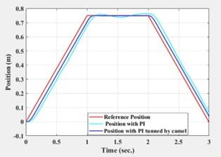
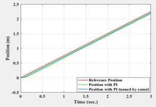
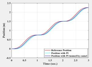
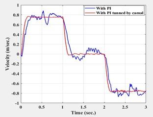
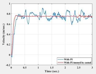
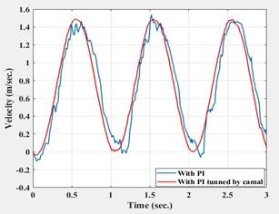
Due to technical limitations in the motor to which position control is applied, various types of reference position trajectories are required for position control. In order to prevent a number of problems, including loss of accuracy, early wear of the machine's parts, and excessive vibration, and the operational limitations of the machine must be observed. To investigate the ability of the motor to track the position trajectory, three different position reference position responses for various suggested reference position trajectories are used which change linearly and non-linearly with time. Figures 9-11 show the linear reluctance motor's trajectories. These figures show that the motor is capable of a quick reaction with a reference position trajectory in both linear and non-linear situations. Moreover, utilizing the CAMEL method for the various kinds of trajectories shown in Figures 12-14 improved the velocity response.
Figure 9. Position response with trapezoidal reference position trajectory
Figure 10. Position response with linear reference position trajectory
Figure 11. Position response with non-linear reference position trajectory
Figure 12. Velocity response with trapezoidal reference position trajectory
Figure 13. Velocity response with linear reference position trajectory
Figure 14. Velocity response with non-linear reference position trajectory
This study uses the MCTA-based PI controller to enhance the trajectory of the LSRM's position. According to the three different reference position trajectory types, Table 3 displays the inaccuracies in the LSRM's location. Position error is represented by the maximum difference between reference position and actual position. The results demonstrate that one of the best ways to enhance the position profile for LSRM is to use the MCTA-based PI controller. The usage of these motors in more applications including high-speed trains, elevators, electromagnetic aircraft launch systems, etc. means that the velocity error must be reduced, and a reduction in tracking position error is crucial. For future work it can be used this algorithm in cascade operation controller of several LSRMs to use in industrial applications.
Table 3. Position error
|
Reference Position Trajectory |
Position Error with PI Controller |
Position Error with MCTA Based PI Controller |
|
Trapezoidal |
0.083 |
0.045 |
|
Linear |
0.083 |
0.045 |
|
Non-linear |
0.1382 |
0.0863 |
[1] Commins, P.A., Moscrop, J.W., Cook, C.D. (2015). Synchronous reluctance tubular linear motor for high precision applications. In 2015 Australasian Universities Power Engineering Conference (AUPEC), Wollongong, Australia, pp. 1-6. https://doi.org/10.1109/AUPEC.2015.7324852
[2] Liu, T., Saho, J., Gao, J., Zhang, L. (2016). Servo system design of direct-drive aerospace linear electro-mechanical actuator. In 2016 IEEE Information Technology, Networking, Electronic and Automation Control Conference, Chongqing, China, pp. 576-580. https://doi.org/10.1109/ITNEC.2016.7560426
[3] Qiu, L., Shi, Y., Pan, J., Xu, G. (2016). Networked H∞ controller design for a direct-drive linear motion control system. IEEE Transactions on Industrial Electronics, 63(10): 6281-6291. https://doi.org/10.1109/TIE.2016.2571263
[4] Bruzzese, C., Rafiei, M., Teodori, S., Santini, E., Mazzuca, T., Lipardi, G. (2017). Electrical, mechanical and thermal design by multiphysics simulations of a permanent magnet linear actuator for ship rudder direct drive. In 2017 AEIT International Annual Conference, Cagliari, Italy, pp. 1-6. https://doi.org/10.23919/AEIT.2017.8240579
[5] Zhang, N., Collins, M., Lovatt, H. (2017). A direct-drive, linear actuator for a heliostat tracking system. In 2017 20th International Conference on Electrical Machines and Systems (ICEMS), Sydney, Australia, pp. 1-5. https://doi.org/10.1109/ICEMS.2017.8055978
[6] El-Touni, H.M., El-Nemr, M.K., Rashad, E.E.M. (2019). Thrust force characteristics of permanent-magnet-assisted linear synchronous reluctance machines using finite element analysis. In 2018 Twentieth International Middle East Power Systems Conference (MEPCON), Cairo, Egypt, pp. 998-1003. https://doi.org/10.1109/MEPCON.2018.8635235
[7] Li, Y., Huang, L., Chen, M., Tan, P., Hu, M. (2021). A linear-rotating axial flux permanent magnet generator for direct drive wave energy conversion. In 2021 IEEE International Magnetic Conference (INTERMAG), LYON, France, pp. 1-5. https://doi.org/10.1109/INTERMAG42984.2021.9579908
[8] Zhi, F., Zhang, M. (2014). Design and analysis of ironless permanent magnet linear synchronous motor with little force ripples for ultra-precision positioning systems. In Proceedings - ASPE 2014 Annual Meeting, pp. 389-394.
[9] Zhang, L., Kou, B., Jin, Y., Chen, Y., Liu, Y. (2016). Investigation of an ironless permanent magnet linear synchronous motor with cooling system. Applied Sciences (Switzerland), 6(12): 5-8. https://doi.org/10.3390/app6120422
[10] Wang, S., Wu, Z., Peng, D., Li, W., Zheng, Y. (2019). Embedded position estimation using tunnel magnetoresistance sensors for permanent magnet linear synchronous motor systems. Measurement: Journal of the International Measurement Confederation, 147: 106860. https://doi.org/10.1016/j.measurement.2019.106860
[11] Garcia-Amorós, J. (2018). Linear hybrid reluctance motor with high density force. Energies, 11(10): 2805. https://doi.org/10.3390/en11102805
[12] Jin, H., Zhao, X. (2019). Approach Angle-Based Saturation Function of Modified Complementary Sliding Mode Control for PMLSM. IEEE Access, 7: 126014-126024. https://doi.org/10.1109/ACCESS.2019.2939140
[13] Yang, R., Li, L., Wang, M., Zhang, C. (2021). Force ripple compensation and robust predictive current control of PMLSM using augmented generalized proportional-integral observer. IEEE Journal of Emerging and Selected Topics in Power Electronics, 9(1): 302-315. https://doi.org/10.1109/JESTPE.2019.2938268
[14] Fu, D., Zhao, X., Yuan, H. (2021). High-precision motion control method for permanent magnet linear synchronous motor. IEICE Electronics Express, 18(9): 1-6. https://doi.org/10.1587/ELEX.18.20210097
[15] Zhou, Y., Zong, W., Tan, Q., Hu, Z., Sun, T., Li, L. (2021). End effect analysis of a slot-less long-stator permanent magnet linear synchronous motor. Symmetry, 13(10): 1939. https://doi.org/10.3390/sym13101939
[16] Pupadubsin, R., Chayopitak, N., Nulek, N., Kachapornkul, S., Jitkreeyarn, P., Somsiri, P., Karukanan, S., Tungpimolrut, K. (2011). Position control of a linear variable reluctance motor with magnetically coupled phases. ECTI Transactions on Electrical Engineering, Electronics, and Communications, 9(1): 195-201.
[17] Chen, S.Y., Chiang, H.H., Liu, T.S., Chang, C.H. (2019). Precision motion control of permanent magnet linear synchronous motors using adaptive fuzzy fractional-order sliding-mode control. IEEE/ASME Transactions on Mechatronics, 24(2): 741-752. https://doi.org/10.1109/TMECH.2019.2892401
[18] Wang, S., Wu, Z., Peng, D., Li, W., Zheng, Y. (2019). Embedded position estimation using tunnel magnetoresistance sensors for permanent magnet linear synchronous motor systems. Measurement: Journal of the International Measurement Confederation, 147: 106860. https://doi.org/10.1016/j.measurement.2019.106860
[19] Shi, X., Lan, Y. (2022). Improved predictive position control for linear synchronous motor with disturbance observer. IEICE Electronics Express, 19(20): 1-6. https://doi.org/10.1587/elex.19.20220375
[20] Štumberger, G., Štumberger, B., Dolinar, D. (2007). Analysis of cross-saturation effects in a linear synchronous reluctance motor performed by finite elements method and measurements. In EPE-PEMC 2006: 12th International Power Electronics and Motion Control Conference, Proceedings, pp. 1907-1912. https://doi.org/10.1109/EPEPEMC.2006.283138
[21] Abdul-Hassan, K.M. (2012). Synchronized position control of dual-linear reluctance motor drive. University of Basrah.
[22] Alawan, M.A., Al-Subeeh, A.N.N., Al-Furaiji, O.J.M. (2019). Simulating an induction motor multi-operating point speed control using PI controller with neural network. Periodicals of Engineering and Natural Sciences, 7(3): 1478-1485. https://doi.org/10.21533/pen.v7i3.784
[23] Kunjittipong, N., Kongkanjana, K., Khwan-On, S. (2020). Comparison of fuzzy controller and PI controller for a high step-up SingleSwitch boost converter. In 2020 3rd International Conference on Power and Energy Applications (ICPEA), Busan, Korea (South), pp. 94-98. https://doi.org/10.1109/ICPEA49807.2020.9280118
[24] Azid, S.I., Shankaran, V.P., Mehta, U. (2020). Fractional PI controller for integrating plants. In 2020 16th International Conference on Control, Automation, Robotics and Vision (ICARCV), Shenzhen, China, pp. 904-909. https://doi.org/10.1109/ICARCV50220.2020.9305506
[25] Bounasla, N., Barkat, S. (2020). Optimum design of fractional order PI speed controller for predictive direct torque control of a sensorless five-phase permanent magnet synchronous machine (PMSM). Journal Europeen des Systemes Automatises, 53(4): 437-449. https://doi.org/10.18280/jesa.530401
[26] Altalabani, W., Alaiwi, Y. (2022). Optimized adaptive PID controller design for trajectory tracking of a quadcopter. Mathematical Modelling of Engineering Problems, 9(6): 1490-1496. https://doi.org/10.18280/mmep.090607
[27] Alkhammash, H.I., Satti, L.M., Ahmad, N., Althobaiti, A., Ullah, N., Babqi, A.J., Ibeas, A. (2023). Optimization of proportional resonant and proportional integral controls using particle swarm optimization technique for PV grid tied inverter. Mathematical Modelling of Engineering Problems, 10(1): 23-30. https://doi.org/10.18280/mmep.100103
[28] Ali, R.S., Alnahwi, F.M., Abdullah, A.S. (2019). A modified camel travelling behaviour algorithm for engineering applications. Australian Journal of Electrical and Electronics Engineering, 16(3): 176-186. https://doi.org/10.1080/1448837X.2019.1640010
[29] Ali, R., Mahmood, J., Badr, H. (2022). A new version of modified camel algorithm for engineering applications. In Proceedings of 2nd International Multi-Disciplinary Conference Theme: Integrated Sciences and Technologies, IMDC-IST 2021, Sakarya, Turkey. https://doi.org/10.4108/eai.7-9-2021.2314874