Mohamed Maniana*![]() | Azddine Azim | Fouad Erchiqui
| Azddine Azim | Fouad Erchiqui![]() | Abdelali Tajmouati
| Abdelali Tajmouati
© 2024 The authors. This article is published by IIETA and is licensed under the CC BY 4.0 license (http://creativecommons.org/licenses/by/4.0/).
OPEN ACCESS
In order to improve the performance and mechanical strength of metal parts, manufacturers often need to perform surface heat treatments on these parts. This work requires a lot of experience and prototyping. The objective of our research work is to develop a numerical calculation method using the principles of heat treatment to predict the desired mechanical characteristics and performance in metal parts without any prior experience. This will help manufacturers to reduce a lot of energy and material. The methodology of this work is based on heat transfer laws and heat treatment diagrams: Time-temperature transformation (TTT) and continuous cooling transformation (CCT). Depending on the heating time and the amount of energy applied to the surface of the metal part, we deduce the metallurgical structure and the hardness (HV) that will manifest itself after heating and cooling of this part.
surface quenching, thermal, mechanical, metallurgy, XC42 steel, numerical, simulation
The objective of our research work is to develop a numerical calculation method using the principles of heat treatment to predict the desired mechanical characteristics and performance in metal parts without any prior experience.
This will help manufacturers to reduce a lot of energy and material, generally wasted in the manufacture of samples and the time allotted for experiment testing.
Manufacturers of metal parts expend a lot of energy and materials to achieve a suitable metallurgical structure that allows this part to have good strength and a long service life in a mechanical system. So, the numerical prediction of this metallurgy will considerably reduce the cost of manufacturing mechanical parts.
Heat treatments are a set of combined heating and cooling operations consisting of austenitization, quenching and tempering.
The heat treatments do not apply to pure metals, but only to a few alloys for which an increase in yield strength and a decrease in brittleness are mainly sought. Heat treatments are applied mainly to XC steels and ZR alloy steels non-ferrous alloys. In general, heat treatments do not change the chemical composition of the alloy. A heat treatment generally allows:
Industrial surface treatment can be provided by several techniques, among which we can mention:
Currently laser technology is highly developed and finds high-level applications in many fields among which we can mention: modern medicine, the pharmaceutical industry and especially the manufacturing industry. This is due to the development of laser beam production devices from the point of view of power, precision and adjustment of the intensity distribution of focalized radiation on the surface of the material to be heated with a temperature adapted to the technological processes selected in the case of surface heat treatment.
The most commonly used process is the martensitic quenching process which is applied to carbon steels and cast irons. The application of the laser beam increases the surface temperature very rapidly (up to 1000℃/s), which transforms the surface layer into austenite. Rapid cooling caused by thermal conduction in the mass of the part, then leads to the martensitic transformation of the steel, generating a very fine microstructure of high hardness. It is important that the steel is in the appropriate conditions (quenched and tempered) and that the processing conditions are carefully selected.
The main advantage of laser tempering is improved wear resistance. Therefore, abrasion wear is reduced to a great extent. Laser-cured surfaces have a higher hardness than the abrasive medium. Adhesion wear can also be influenced by a reduction in the coefficient of friction. In addition, laser quenching can improve surface fatigue characteristics through increased compressive stress, which shifts load capacity to a level higher than the applied wireless stress.
The variation in the absorption coefficient of optical energy influences the quality of the results Altergott and Patel [1] and Zhang et al. [2].
The surface finish mainly affects the absorption of the laser beam. Wisembach et al. [3].
Steel hardening is a fundamental process of metallurgy that improves mechanical characteristics [4-7].
A new modification layer on the surface of ductile iron with a perlite-ferrite matrix was manufactured under irradiation of an Nd:YAG laser beam equipped with a self-designed diffractive optical element (DOE) that produces a two-dimensional microhardness map of higher hardness [8].
During quenching alloying elements can also influence a steel's ability to absorb laser light. Each metal absorbs wavelengths in a different way [9].
The importance of gear wheel design gives priority to scientific research in the heat treatment of gears. The aim was to increase the resistance to wear at the point of contact and bending at the foot of the tooth. In the literature, this treatment is found under the name contour type tempering [10].
Research carried out that specified LHT diagrams for different engineering materials in general. This diagram distinguishes the range of parameters of the laser beam and their effects in the surface layer of gray iron [11].
Simulation of different laser source models in welded material in the case of welding process simulations using solid-state and high-power diode lasers [12].
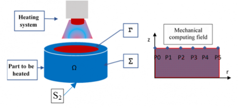
The sample used in this work is an XC42 steel cylinder marked by six points in the surface to be treated and which are diametrically equidistant see Figure 1.
On the upper surface of this cylinder, a heat flux with a Gaussian profile and variable over time is applied to a circular zone with a diameter smaller than the outer diameter of the cylinder.
Figure 1. Physical model
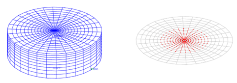
Depending on the high-density energy profile (Figure 2) concentrated in the center of the surface to be treated, we chose a non-regular mesh with a density that varies from 0.002 mm in the center to 0.005 mm at the edge of this surface. To have a better calculation accuracy with the finite element method, we chose a cubic geometric element with 8 nodes and an optimal time step of 0.1 seconds.
Figure 2. Mesh
The sample used in this numerical calculation is a cylindrical part with diameter (d), height (l), total mass (m). The treated area (Γ) is limited by a radius ($\mathrm{R}_L$) of 40 mm. The numerical values of these geometric characteristics are defined in Table 1.
The Vickers hardness (HV), calculated by Eqs. (15)-(17), of each solid phase that appears in the metallurgical composition at the end of the heat treatment of the sample, is highly dependent on the chemical composition of the material chosen for that sample. The composition of our sample (XC42) is defined in Table 2.
Table 1. Sample geometry
|
Quantity |
Value |
|
Diameter (d) [mm] |
100 |
|
Height (l) [mm] |
30 |
|
Mass (m) [kg] |
0.463 |
|
Radius of Heated surface ( $\mathrm{R}_L$ [mm] |
40 |
Table 2. Chemical composition
|
XC42 STEEL |
||||
|
C |
S |
Mn |
P |
Si |
|
0.37 |
0.035 |
0.50 |
0.035 |
0.40 |
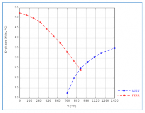
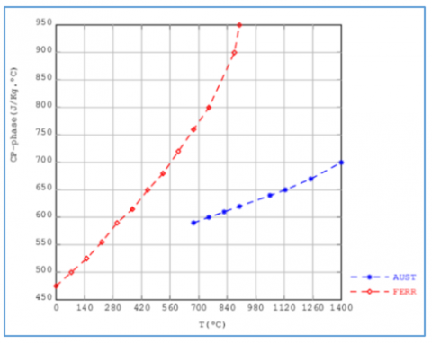
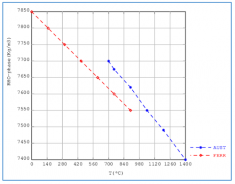
In our numerical calculation model, we have taken into account the evolution of the thermo-physical characteristics: conduction heat exchange coefficient (k), mass heat capacity (cp.) and the volume density (ρ) of the different solid phases: austenite (Aust) and ferrite (Ferr) of the material used, see Figures 3-5.
Figure 3. Thermal conductivity
Figure 4. Thermal capacity
Figure 5. Density
5.1 Thermal problem
Knowing the heat flux $\varphi(r, \theta, z, t)$ applied to the surface $(\Gamma)$, The solution of this mathematical problem consists in the determination of the temperature $T(r, \theta, z, t)$ at any point of the sample and at each step of time.
$\rho c_p \frac{\partial T(r, \theta, z, t)}{\partial t}+\operatorname{div}(-k(T) \cdot \overline{\operatorname{grad}} T(r, \theta, z, t))=0$ in $\Omega$ (1)
The boundary conditions used in this problem are:
$-\left.k(T) \frac{\partial T(t, r, \theta, z)}{\partial n_1}\right|_{z=l}=\varphi(r, \theta, z, t)$ on $\Gamma$ (2)
$-\left.k(T) \frac{\partial T(t, r, \theta, z)}{\partial n_2}\right|_{r=R}=h .\left(T(r, \theta, z, t)-T_{\infty}\right)$ on $\Sigma$ (3)
$-\left.k(T) \frac{\partial T(t, r, \theta, z)}{\partial n_1}\right|_{\substack{r \geq R_L \\ z=l}}=h .\left(T(r, \theta, z, t)-T_{\infty}\right)$ on $\mathrm{S}_1$ (4)
$-\left.k(T) \frac{\partial T(t, r, \theta, z)}{\partial n_3}\right|_{z=0}=0$ on $S_2$ (5)
Initial condition:
$T(r, \theta, z, t)=T_0$ in $\Omega$ at $t=0$ (6)
Metallurgical calculation is developed by Maniana et al. [13] and Maniana et al. [14] in their work on solving the inverse problem during laser heat treatment.
With the concentrations of each element in %m. The second category corresponds to bainitic and ferritic/pearlitic transformations. This modeling is represented by the Johnson-Mehl-Avrami-Kolmogorov equation (JMAK) [15]:
$y_k=y_{\max k}\left[1-e^{-b_k \times t^{n k}}\right]$ (7)
Perlite: k=1, ferrite: k=2, Austenite: k=3.
$y_{\max k}$: Maximum fraction that can be transformed.
$n_k$ and $b_k$: Temperature-dependent parameters.
$n_k(T)=\frac{\log \left[1-y_1\right] / \log \left[1-y_2\right]}{\log \left(t_1 / t_2\right)}$ (8)
$b_k(T)=\frac{\log \left[1-y_1\right]}{t_1^{n k}}$ (9)
$t_k$: Time that corresponds to the processing level of the constituent.
The austenite formation temperatures must be known to ensure complete homogenization during austenitization. It is possible to determine them by dilatometric tests, but prediction using Andrews' empirical formulas is a good estimate [16]:
$\begin{gathered}A \mathrm{c} 1=723-10.7 M n-16.9 N i+29.1 S i+16.9 C r+ 290 A s+638 W\end{gathered}$ (10)
$\begin{gathered}A \mathrm{c} 3=910-203 \sqrt{C}-15.2Ni+44.7 Si+104 V+ 31.5 Mo+13.1 W\end{gathered}$ (11)
Modelling transformations during cooling after austenitization is divided into two categories: Transformation by displacement or transformation by diffusion. The first corresponds only to the martensite which is described by the equation of (K-M) [17].
$y_k=y_{\max k}\left[1-e^{-A_m\left(M_s-T\right)}\right]$ (12)
$A_m$: Koistinen coefficient.
$M_s$: Martensitic transformation start temperature.
$T$: Running temperature.
The Ms is the temperature at which the martensitic transformation begins and T is the temperature at which the martensite fraction wants to be calculated. The temperature at the beginning of the martensitic transformation is calculated using empirical equations, such as Andrews' corrected [18, 19]:
$\begin{gathered}M s\left({ }^{\circ} \mathrm{C}\right)=500-300 \mathrm{C}-33 \mathrm{Mn}-17 \mathrm{Ni}-22 \mathrm{Cr}-11 \mathrm{Si}-11 \mathrm{Mo}\end{gathered}$ (13)
With the concentrations of each element in %m.
One of the equations used to calculate the temperature at the beginning of bainite formation is given by Steven-Haynes [20]:
$\begin{gathered}B S\left({ }^{\circ} \mathrm{C}\right)=830-270 \mathrm{C}-90 \mathrm{Mn}-37 \mathrm{Ni}-70 \mathrm{Cr}- 83 \mathrm{Mo}\end{gathered}$ (14)
Hardness is a good characteristic of the microstructure of an alloy it is interesting to be able to model this property to anticipate transformations during heat treatment. Among the models that allow a prediction of hardness is the equation of Maynier et al. [21] allowing the hardness to be calculated as a function of composition:
$\begin{gathered}H V_M=127+949 \mathrm{C} \%+27 \mathrm{Si} \%+8 N i \%+ \\ 16 \mathrm{Cr} \%+21 \log \left(V_r\right)\end{gathered}$ (15)
$\begin{aligned} H V_B=-323+ & 185 C \%+330 S i \%+135 M n \% \\ & +65 N i \%+144 C r \% \\ & +191 M o \%+(89+53 C \\ & -55 S i+22 M n-10 N i \\ & -20 C r-33 M o) \log \left(V_r\right)\end{aligned}$ (16)
$\begin{gathered}H V_{F / P}=42+223 C \%+533 S i \%+30 M n \% \\ +12.6 N i \%+(10-19 S i+4 N i \\ +8 C r+130 V) \log \left(V_r\right)\end{gathered}$ (17)
where, HVM, HVB and HVF/P are the hardness of martensite, bainite and ferrite/perlite respectively. Vr is the cooling rate in ℃/h.
The mixing law makes it possible to calculate the total hardness of an alloy comprising all these phases by the following relation:
$H V_{T o t}=\left(y_F+y_P\right) H V_{F / P}+y_B H V_B+y_M H V_M$ (18)
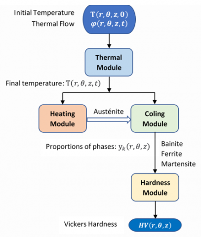
All of these mathematical models described in this paragraph are organized as calculation modules and are represented in the flowchart in Figure 6.
Figure 6. Flowchart of the digital method
The determination of the mechanical characteristic of Vickers hardness is done according to the flowchart in Figure 6.
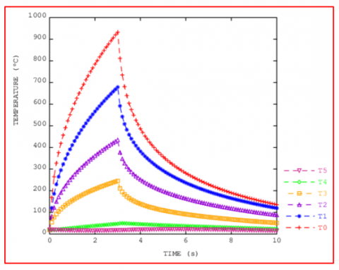
The numerical solution of the heat transfer equation (Eq. (1)) by a thermal module allowed us to know the temperature distribution over the entire computational domain (Ω) that we used to plot the evolution of temperature as a function of time at five points P0-P5.
Figure 7. Temperature at six different points
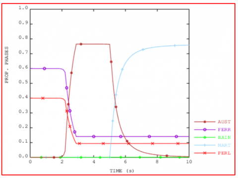
These numerical results allowed us to deduce the maximum temperature reached, the heating rate and the cooling rate at each point of (Ω), by introducing these latter parameters into two modules, the heating and cooling modules, defined on metallurgical models based on Eqs. (7)-(14). These last modules will allow us to calculate the fractions of solid phases (Figures 7 and 8) that can be formed in the material after heating and cooling. Finally, another modulus of hardness using these fractions can tell us about the Vickers hardness (HV) at each point of the material, see Figures 9 and 10.
Figure 8. Evolution of the proportion of phases versus time at point P0
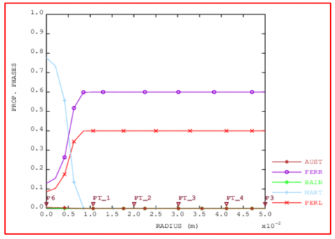
Figure 9. Evolution of the proportion of phases versus radius
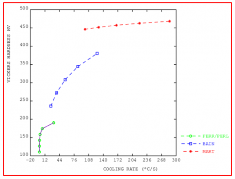
Figure 10. Evolution of the hardness versus cooling rate
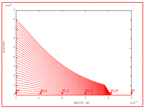
In Figure 11 we have represented the evolution of the heating flow applied in this case of treatment respectively as a function of radius and versus time.
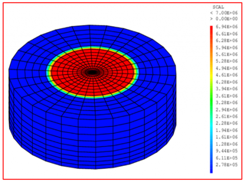
Figure 12 shows the distribution density of the heat flux applied to the treated surface of the sample.
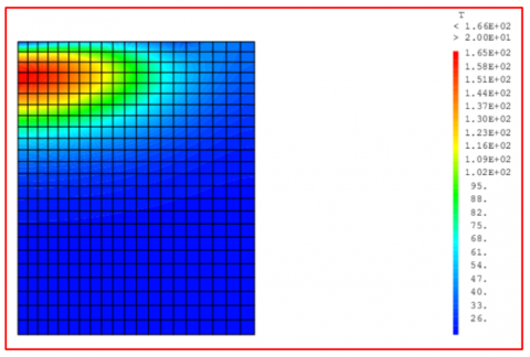
Figure 13 shows the distribution of temperature after cooling.
Figure 7 shows the evolution over time of the surface temperatures taken at six points (numbered from P0 to P5) uniformly distributed over the radius of the upper face of the cylinder.
Figure 11. Distribution of flow versus space end time
Figure 12. Distribution of applied flow density
Figure 13. Distribution of temperature after cooling
In Figure 9 we have represented the distribution of the rates of the solid phases according to the radius of the surface treated, on the other hand Figure 10 represents the evolution of this rate according to the depth of this surface.
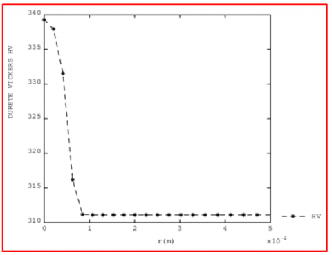
By using the mixing law and knowing the proportions of the solid phases at each point of the radius, this allowed us to estimate the total hardness at any point in the radial direction, see Figure 14.
Hardness is a mechanical characteristic that has a very high bearing in the mechanical resistance to surface friction and penetration.
Figure 14. Evolution of the hardness versus radius
This numerical simulation allowed us to know the temperature mapping at all points of the sample and in particular its distribution in the treatment surface figure 10. It also allowed us to predict the metallurgical structure in the treatment area Figures 9, 10 and 14.
The heat treatment of metal surfaces improves the quality of mechanical characteristics, among which there is hardness which plays an important role in resistance to wear and deformation. To improve the latter, it is necessary to choose an adequate heat treatment cycle with the desired results. This calculation code makes it possible to numerically simulate the heat treatment operation before carrying out the experiment.
This saves a lot of energy and the material generally wasted in experimentation which reduces the cost of realization of mechanical parts by guaranteeing better quality / price.
This numerical method is of great importance in the heat treatment of solid-state phase transformation materials, it allows us to know the hardness at any point of the sample that is impossible to achieve by direct measurement.
|
$\emptyset$ |
Heat flow (W) |
|
$\varphi$ |
Surface heat flow (W.m-2) |
|
$k$ |
Conductivity (W.m-1.K-1) |
|
$\rho$ |
Density (kg.m-3) |
|
$cp$ |
Mass calorific capacity (mass heat) (J.kg-1.K-1) |
|
$h$ |
Convection coefficient (W.m-2.K-1) |
|
HV |
Vickers Hardness |
|
$t$ |
Time (s) |
|
$t_f$ |
final time (s) |
|
R |
Radius (m) |
|
RL |
Radius of the treated surface |
|
$S$ |
Surface (m²) |
|
$T$ |
Temperature (°C) |
[1] Altergott, W., Patel, P. (1982). Bell Helicopter Textron. Spur Gear Laser Surface Hardening MM&T Program. Rapport No. USAAVRADCOM-TR-81-D-47. Fort Eustis, Virginie: Illinois Institute ofTechnology, 120. https://apps.dtic.mil/sti/citations/ADA114670.
[2] Zhang, H., Shi, Y., Xu, C.Y., Kutsuna, M. (2003). Surface hardening of gears by laser beam processing. Surface Engineering, 19(2): 134-136. https://doi.org/10.1179/026708403225002595
[3] Wissenbach, K. Gillner A. Dausinger F. (1985). Transformation hardening by CO2 laser radiation. Laser and Optoelectronic, 3: 291-296. https://publica.fraunhofer.de/search?query=Wissenbach,%20K.%20Gillner%20A.%20Dausinger%20F.%201985.
[4] Unterweiser, P.M., Boyer, H.E., Kubbs. (1982). Heat Treater's Guide (Standard Practices and Procedures for Steel, 2 Edition. Colombus, Ohio, US: ASM International. https://www.abebooks.fr/9780871701411/Heat-Treaters-Guide-Standard-Practices-0871701413/plp.
[5] ASM International Handbook Committee. (1991). Heat Treating. Collection. Metals Handbook, Volume 4. Cleveland: American Society for Metals, 217. https://www.standardsmedia.com/ASM-Handbook-Volume-4--Heat-Treating-2448-book.html.
[6] Chandler, H. (1995). Heat Treater's Guide: Practices and Procedures for Irons and Steels, 2end Edition. Columbus, Ohio, US: ASM International. https://www.amazon.com/Heat-Treaters-Guide-Practices-Procedures/dp/B013RO1GL2
[7] Davis, R. (2002). Surface Hardening of Steels: Understanding the Basics. ASM International, 364. https://www.asminternational.org/surface-hardening-of-steels-understanding-the-basics/results//journal_content/ 56/06952G/ PUBLICATION/.
[8] Yang, L.J., Cheng, K.H. (2001). Laser transformation hardening of steel. South East Asia Iron and Steel Institute Quarterly, 30(4): 42-49.
[9] Donald, R., Pradeep, P.F., Wendelin, W. (2010). The Science and Engineering of Materials. 6e édition. Stamford, CT: Cengage Learning, 944. https://www.amazon.com/Science-Engineering-Materials-Donald-Askeland/dp/0495296023.
[10] Austin, Samuel. Étude Expérimentale de la Résistance à la Flexion en Pied de Dent de Roues Droites Cylindriques Traitées Thermiquement Par Induction. Rimouski, QC: Université du Québec à Rimouski, 230. https://semaphore.uqar.ca/id/eprint/720.
[11] Paczkowska, M. (2016). The evaluation of the influence of laser treatment parameters on the type of thermal effects in the surface layer microstructure of gray irons. Optics and Laser Technology, 76: 143-148. https://doi.org/10.1016/j.optlastec.2015.07.016
[12] Kik, T. (2020). Heat source models in numerical simulations of laser welding. Materials, 13(11): 2653. https://doi.org/10.3390/ma13112653
[13] Maniana, M., Azim, A., Rhanim, H., Archambault, P. (2009). Problème inverse pour le traitement laser des métaux à transformations de phases. International Journal of Thermal Sciences, 48(4): 795-804. https://doi.org/10.1016/j.ijthermalsci.2008.05.018
[14] Maniana, M., Azim, A., Erchiqui, F., Tajamouati, A. (2022). Reconstruction of the thermal source from the temperature measured case of surface heat treatment of steel by laser beam. International Journal of Heat and Technology, 40(6): 1507-1513. https://doi.org/10.18280/ijht.400620
[15] Johnson, W.A., Mehl, R.F. (1939). Transactions, American Institute of Mining and Metallurgical Engineers. the Institute., New York, 416. https://www.abebooks.com/Transactions-American-Institute-Mining-Metallurgical-Engineers/30295701504/bd.
[16] Dobrzański, L.A., Trzaska, J. (2004). Application of neural networks to forecasting the CCT diagrams. Journal of Materials Processing Technology, 157-158: 107-113. https://doi.org/10.1016/j.jmatprotec.2004.09.009
[17] Wilson, E.A., Medina, S.F. (2000). Application of Koistinen and Marburger’s athermal equation for volume fraction of martensite to diffusional transformations obtained on continuous cooling 0·13%C high strength low alloy steel. Materials Science and Technology, 16(6): 630-633. http://doi.org/10.1179/026708300101508397
[18] Sourmail, T., Smanio, V. (2014). Response to A second set of comments on “Determination of Ms temperature: Methods, meaning and influence of the ‘slow-start’ phenomenon". Science and Technology, 30(4): 511-512. https://doi.org/10.1179/1743284713Y.0000000417
[19] Bouissa, Y., Zorgani, M., Shahriari, D., Champliaud, H., Morin, J.B., Jahazi, M. (2021). Microstructure-based FEM modeling of phase transformation during quenching of large-size steel forgings. Metallurgical and Materials Transactions A, 52(5): 1883-1900. https://doi.org/10.1007/s11661-021-06199-4
[20] Lee, Y.K. (2002). Empirical formula of isothermal bainite start temperature of steels. Journal of Materials Science Letters, 21: 1253-1255. https://doi.org/10.1023/A:1016555119230
[21] Maynier, P., Dollet, J., Bastien, P. (1978). Hardenability Concepts with Application to Steel, D.V. Doane and J.S. Kirkaldy, eds., TMS-AIME, Warrendale, 163. https://books.google.co.ma/books/about/Hardenability_Concepts_with_Applications.html?id=8spTAAAAMAAJ&redir_esc=y.