Bala Srinivas Peteti*![]() | Durgesh Nandan
| Durgesh Nandan![]()
(This article is part of the Special Issue: Technology Innovations and AI Technology in Healthcare)
© 2023 IIETA. This article is published by IIETA and is licensed under the CC BY 4.0 license (http://creativecommons.org/licenses/by/4.0/).
OPEN ACCESS
Heart disease is the biggest cause of death worldwide; it cannot be seen with the bare eyes and occurs suddenly when its limits are reached. It requires a correct diagnosis at the right moment. Every day, the health care sector generates a massive amount of data about patients and diseases. However, scholars and practitioners do not make effective use of this data. The healthcare sector is currently data-rich but knowledge-poor. To effectively extract information from databases and apply that knowledge for diagnosis that is even more precise and decision-making, a variety of data mining and machine learning approaches and technologies are available. As research on algorithms for predicting heart disease expands, it is critical to assess the findings, which are now unclear. The primary purpose of this research paper is to present a summary of current research on the use of datasets, classifiers, data preprocessing methods, and the efficiency of integrating both to predict heart disease, with comparison findings and analytical conclusions. According to the study, the performance of the heart disease prediction system is improved in many scenarios by the use of KNN, ANN, RF, PCA, χ 2 and GA algorithms.
heart disease, classifier, data preprocessing, heart disease datasets, machine learning, deep learning, review, prediction
Heart disease (HD) refers to a wide range of heart-related medical problems. These medical diseases explain abnormalities that have a direct impact on the heart and all of its parts. Heart disease is currently a serious public health concern. HD or cardiovascular disease (CVD) is that the leading reason for a death worldwide. In line with world statistics, 17.9 million people die every year from HDs. HD causes more than 32% of global deaths each year. It is estimated that more than 130 million adults will have HD by 2035 [1]. HD is a group of heart and vascular diseases, including ischemic HD, cerebrovascular disease, rheumatic HD, and other conditions. The main behavioral risk factors for HD and stroke are poor diet, sedentary lifestyle and tobacco use, and harmful effects [2]. Quitting smoking, reducing the salt content in your diet, eating more fruits and vegetables, exercising regularly, and avoiding harmful drinks have been shown to reduce your risk of HD. It is crucial to identify HD as early as possible. Possible for people at increased risk for HD and ensuring adequate treatment can prevent premature deaths [3]. However, accurate diagnosis is difficult to achieve and is frequently delayed due to the numerous factors that complicate disease diagnosis [4].
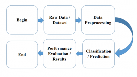
The Heart Disease Data Prediction is made to help doctors make accurate diagnoses of heart disease. They usually do their work using a knowledge foundation of clinical competence and a study of medical data. Improvements to these Predicting algorithms can raise the calibre of medical diagnoses for heart disease [5]. A method for extracting the information buried in the data is data mining [6]. Data mining is a process of data processing used to find hidden patterns in massive amounts of data. It's been successfully applied to information retrieval in a variety of fields [7]. According to Giudici, it is a process of exploration, collecting, and analysis of enormous amounts of data to reveal patterns and interconnections that are initially unknown with the purpose of finding obvious and useful information for the authorities of database. Various data mining techniques have been utilized and developed in the modern era [8]. In recent years, we have seen growth in all fields and in almost all data types. In recent years, the growth of biomedical data has been particularly rapid due to the exponential growth in knowledge in the biomedical field [9]. With the help of knowledge discovery or data mining (DM) methods based on different machine learning (ML) and deep learning (DL) methods, it is possible to determine predictive models from different sources of medical data as well as the predictive accuracy of the resulting smart data [10]. The system can even be very precise. It is a process of finding the correlation or pattern between different regions in a large medical database. Affected by the annual increase in the global death rate of patients with heart disease (HD) and the large amount of patient data available. Researchers use data mining to help healthcare providers manage their conditions by providing them with vital information [11]. This motivates us to conduct this review of studies examining classifiers and classifiers using data preprocessing techniques in predicting HD. Figure 1 shows the Simple experimental workflow of heart disease prediction.
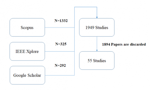
The goal of this review is therefore to empirically examine the effectiveness of classifiers and classifiers with data preprocessing in the prediction / classification of HDs. The evaluation recognized applicable research published between 2007 and 2020, leading to a complete of 55 researches. From this research, we recall the most effective ones that could be associated with practicing HD data for the purpose of classification. Highlight the fact that, the primary research have been recognized the use of the subsequent search string: (TITLE-ABS-KEY ("heart disease" OR "cardiovascular disease") AND TITLE-ABS-KEY ("prediction" OR “classification”) AND TITLE-ABS-KEY ("machine learning" OR "deep learning").This search string became utilized in 3 virtual databases namely: Scopus database, IEEE Xplore virtual library and Google Scholar. Figure 2 shows the study selection of the outcomes of the choice manner of this review. General primary research from 1949 published between 2007 and 2020 was recognized using virtual searchable databases. Of the 1,949 articles, 55 articles were selected that focused on the use of classifiers in predicting / classifying HD.
Figure 1. Simple experimental workflow of heart disease prediction
The reason for this review has been changed to compile and summarise the empirical proof regarding the applying of classifiers and classifiers with data preprocessing strategies in predicting / classifying HD by answering five questions: (1) Identify the datasets used for prediction of HD, (2) Identify the classifiers used for prediction of HD, (3) Identify the classifiers which provide the higher overall performance in HD classification, (4) Identify the data pre-processing techniques in combination with classifiers utilized in HD classification, and (5) Identify which combinations of classifiers with data pre-processing techniques are good on the utility of HD prediction.
The paper follows the following structure: The datasets used for HD prediction are described in Section 2. Most commonly used performance metrics to evalute the efficiency of the system are given in Section 3. Several classifiers utilised in HD prediction are then given in section 4. The data pre-processing techniques are described in Section 5. The combination of classifier with data preprocessing techniques are described in section 6. Section 7 includes conclusion & future scope.
Figure 2. Result of study selection process
A dataset is a group of observations saved in a tabular layout wherein every row is one observation and wherein every column incorporates a data factor that relates to a feature of an observation. Data units can maintain facts consisting of scientific data or insurance data, to be utilized by a application running at the machine. Data units also are used to keep information wanted through programs or the working machine itself, consisting of source programs, macro libraries, or machine variables or parameters. Datasets are essential to foster the improvement of numerous computational fields, giving scope, robustness, and self-assurance to results. Datasets have become famous with the evolution of artificial intelligence, machine learning, and deep learning. In Machine Learning, you can divide your data into training, testing, and validation datasets. A dataset is frequently utilised for purposes other than educational. A training dataset that has been processed is commonly cut up into multiple pieces in order to test how well the model's training went [12].
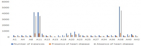
In the early prediction/classificatin of HD 42 plus datasets are used and those datasets are tabulated in Table 1 and corresponding charts are shown in Figure 3. In Table 1, name of the dataset, number of instances, number of attributes, presence of HD, absence of HD and missing values are arranged as contents of the columns. Among these 42 plus datasets 3 datasets are mostly used. They are, Statlog HD dataset (270), Cleveland HD dataset (297) and Cleveland HD dataset (303).
Figure 3. Representation for dataset corresponding to number of instances, presence of heart disease and absence of heart disease
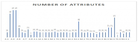
Figure 4. Representation of dataset corresponding to number of attributes
Table 1. Datasets used for heart disease prediction/ classification
|
Dataset code |
Name of the data set |
Number of instances |
Number of attributes |
Presence of heart disease |
Absence of heart disease |
Missing values |
Reference |
|
A1 |
Cleveland heart disease dataset |
297 |
14 |
137 |
160 |
No |
[2, 5, 13 -18] |
|
A2 |
Cardiovascular disease dataset |
3000 |
66 |
- |
- |
No |
[4] |
|
A3 |
Cleveland heart disease dataset (unprocessed) |
303 |
76 |
139 |
164 |
Yes |
[6] |
|
A4 |
Heart Disease Data.arff |
303 |
76 |
120 |
150 |
No |
[6] |
|
A5 |
Indira Gandhi Medical College (IGMC), Shimla CAD dataset |
335 |
26 |
- |
- |
Yes |
[7] |
|
A6 |
Cleveland heart disease dataset |
303 |
14 |
139 |
164 |
Yes |
[8, 10, 19-33] |
|
A7 |
Heart disease 2 dataset |
23 |
12 |
- |
- |
No |
[10] |
|
A8 |
SPECT dataset |
267 |
22 |
223 |
49 |
No |
[24] |
|
A9 |
Eric dataset |
209 |
7 |
- |
- |
No |
[24] |
|
A10 |
Framingham dataset |
4238 |
16 |
643 |
3595 |
Yes |
[33] |
|
A11 |
Heart Disease dataset |
4238 |
16 |
643 |
3595 |
Yes |
[33] |
|
A12 |
Cleveland and Hungarian heart disease dataset |
577 |
14 |
345 |
232 |
No |
[34] |
|
A13 |
Cleveland heart disease dataset |
283 |
14 |
157 |
126 |
No |
[34-35] |
|
A14 |
Hungarian heart disease dataset |
294 |
14 |
188 |
106 |
No |
[35] |
|
A15 |
Switzerland heart disease dataset |
123 |
14 |
115 |
8 |
Yes |
[35] |
|
A16 |
Hungarian heart disease dataset |
294 |
14 |
106 |
188 |
Yes |
[34-36] |
|
A17 |
Kita Hospital Jakarta (HKH) dataset |
450 |
16 |
- |
- |
No |
[36] |
|
A18 |
Health insurance research database of Taiwan nation (NHI database) |
317 |
13 |
84 |
233 |
No |
[36] |
|
A19 |
Cleveland, Hungarian heart disease dataset |
597 |
14 |
245 |
352 |
Yes |
[36] |
|
A20 |
Cleveland, Hungary, and Switzerland datasets |
720 |
14 |
360 |
360 |
Yes |
[36] |
|
A21 |
Cleveland, Long Beach VA, Switzerland, and Hingarian dataset |
920 |
14 |
509 |
411 |
Yes |
[36] |
|
A22 |
Rajaie cardiovascular medical dataset |
303 |
13 |
- |
- |
No |
[36] |
|
A23 |
Cleveland and Statlog heart disease dataset |
573 |
14 |
259 |
314 |
Yes |
[36] |
|
A24 |
Cleveland heart disease dataset |
270 |
14 |
120 |
150 |
No |
[37, 38] |
|
A25 |
SPECTF dataset |
267 |
44 |
223 |
49 |
No |
[38] |
|
A26 |
Heart disease dataset (catalog) |
270 |
14 |
120 |
150 |
No |
[38] |
|
A27 |
Statlog heart disease dataset |
270 |
13 |
120 |
150 |
No |
[39-45] |
|
A28 |
Cleveland heart disease dataset |
296 |
14 |
136 |
160 |
No |
[41] |
|
A29 |
Heart disease 1 dataset |
40 |
12 |
- |
- |
No |
[42] |
|
A30 |
Heart disease Andhra Pradesh |
23 |
12 |
- |
- |
No |
[43] |
|
A31 |
Heart disease Andhra Pradesh |
768 |
9 |
- |
- |
No |
[43] |
|
A32 |
Heart Disease dataset |
10082 |
14 |
- |
- |
Yes |
[46] |
|
A33 |
Heart Disease dataset |
81 |
14 |
- |
- |
No |
[46] |
|
A34 |
Long Beach VA heart disease dataset |
200 |
14 |
149 |
51 |
Yes |
[47] |
|
A35 |
SDS data set |
335 |
27 |
164 |
171 |
Yes |
[48] |
|
A36 |
CDS data set |
335 |
27 |
164 |
171 |
Yes |
[48] |
|
A37 |
Z-Alizadeh Sani CHD dataset |
303 |
55 |
216 |
87 |
No |
[49] |
|
A38 |
Cardiovascular disease dataset |
5209 |
7 |
689 |
4520 |
No |
[50] |
|
A39 |
Heart disease (angina) dataset |
270 |
14 |
120 |
150 |
No |
[51] |
|
A40 |
South Africa HD dataset |
462 |
10 |
160 |
302 |
No |
[52] |
|
A41 |
Cleveland and VA Long Beach heart disease dataset |
503 |
14 |
288 |
215 |
Yes |
[53] |
|
A42 |
Heart disease dataset |
300 |
14 |
140 |
160 |
Yes |
[54] |
Cleveland HD dataset (303) contains 14 attributes, 303 instances with 139 presence and 164 absences [55]. The "goal" field indicates whether the patient has HD or not. Integer values range from 0 to 4. While experimenting with the Cleveland database, the focus has been on attempting to differentiate between presence of HD (values 1,2,3,4) and absence of HD (value 0) [13, 19]. Statlog HD dataset (270) is multivariate and this database contains 13 attributes, 270 instances with 120 presence and 150 absences [34]. Cleveland HD dataset (297) contains 14 attributes, 297 instances with 137 presence and 160 absences. The "goal" field indicates whether the patient has HD or not. Integer values range from 0 to 4. While experimenting with the Cleveland database, the focus has been on attempting to differentiate between presence of HD (values 1,2,3,4) and absence of HD (value 0) [37]. These 3 datasets are gathered from the UCI machine learning repository. Generally, most of the datasets can be download from Kaggle and GitHub. The datasets corresponding attributes are shown in Figure 4.
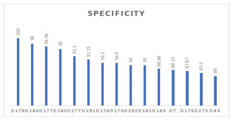
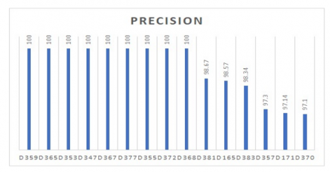
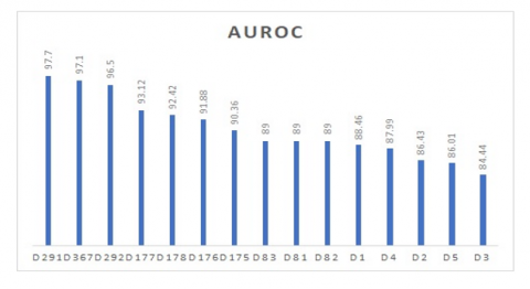
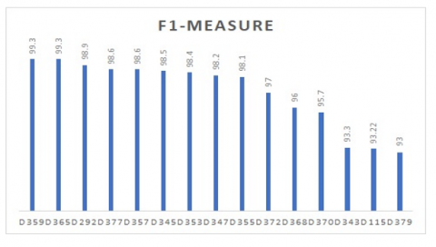
Usually, performance of any physical quantity/matter can be considered as productive based on different parameters. The most used Performance metrics for classification problems are Accuracy, Sensitivity, Specificity, Precision, F1-Score, Area under the receiver operator curve [20]. The listed variables are subjected to different algorithm techniques to compare and analyse the efficiency.
3.1 Accuracy (ACC)
Accuracy is described as the percentage of correct predictions of the experimental data. It is easy to calculate by splitting the number of correct guesses by the total number of guesses. More formally, it is described as the number of true positive and true negative results divided by the number of true positive, true negative, false and false negative results. If you are solving a classification problem, the best result is 100% accuracy. If you are solving a regression problem, the best result is an error of 0.0%. These estimates are unattainable upper / lower limits. All predictive modelling problems contain forecast errors [56].
$Accuracy$ $=\frac{ { correctly \,predicted \,class }}{ { total\, testing\, class }} \times 100 \%$ (1)
(OR)
As the proportion of effectively categorized instances
$Accuracy$ $=\frac{(T P+T N)}{(T P+T N+F P+F N)}$ (2)
where, TP, FN, FP and TN represent the number of true positives, false negatives, false positives and true negatives, respectively.
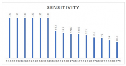
3.2 Sensitivity, hit rate, recall, or True Positive Rate (TPR)
Sensitivity could be a live of the proportion of actual positive cases that got foreseen as positive (or true positive). Sensitivity is outlined as the true-positive recognition rate: number of true positives / (number of true positives + number of false negatives). This means, what percentage subjects with a sickness are literally known as having the disease by the test [56].
$Sensitivity$ $=\frac{T P}{(T P+F N)}$ (3)
3.3 Specificity, selectivity or True Negative Rate (TNR)
Specificity is outlined because the proportion of actual negatives, that got foreseen as the negative (or true negative). This means that there'll be another proportion of actual negative, which got predicted as positive and will be termed as false positives. This proportion could even be referred to as a false positive rate. In different words, it represents the proportion of individuals while not the disease, that may have a negative result [56].
$Specificity$ $=\frac{T N}{(T N+F P)}$ (4)
3.4 Precision or Positive Predictive Value (PPV)
Precision (also referred to as positive predictive value) is that the fraction of relevant instances among the retrieved instances. preciseness may be a live that tells us out of all expected cases, what number are actual cases potential values vary from zero to one [19].
$Precision$ $=\frac{T P}{(T P+F P)}$ (5)
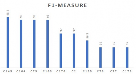
3.5 F1-Score
The F1 Score is additionally referred to as the F Score or the F Measure. place another way, the F1 score conveys the balance between the exactitude and therefore the recall. The F1-score is the mean between precision and recall. during this case, we aim for each high recall and high precision, that means we wish to be able to determine an oversized variety of cases and that we also want to make sure that the bulk of foreseen cases are actual cases. The F1-score ranges from zero to one, wherever 0 is the worst performance [56].
$F_{1-}$Score $=2 * \frac{({ Precision } * { Recall })}{( { Precision }+ { Recall })}$ (6)
(OR)
$F_{\beta_{-}}$Score $=\left(1+\beta^2\right) \frac{ { Precision } * { Recall }}{\left(\beta^2 * { Precision }\right)+ { Recall }}$ (7)
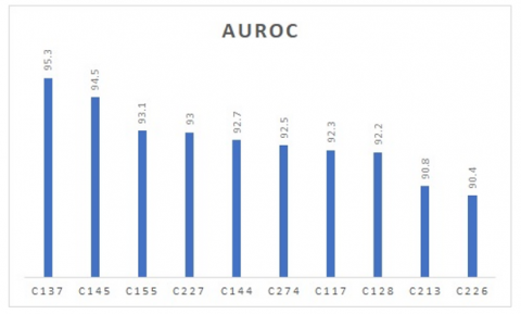
3.6 Area under the receiver operator curve (AUROC)
AUROC curve may be a performance measure for the classification issues at numerous threshold settings. ROC is a probability curve and AUC represents the degree or measure of separability. It tells what proportion the model is capable of distinctive between categories. Higher the AUC, the higher the model is at predicting zero classes as 0 and one classes as 1. By analogy, the upper the AUC, the better the model is at distinguishing between patients with the illness and no disease. The AUC for the roc will be calculated by using the roc_auc_score(). Just like the roc_curve() function, the AUC function takes both the true outcomes (0,1) from the check set and therefore the foreseen chances for the one class. It returns the AUC score between zero and one for no ability and excellent skill respectively [56].
Some of the other parameters used to measure the performance of a classification model are Negative Predictive Value (NPV), Miss Rate or False Negative Rate (FNR), Fall-Out or False Positive Rate (FPR), False Discovery Rate (FDR), False Omission Rate (FOR), Positive Likelihood Ratio (LR+), Negative Likelihood Ratio (LR-) and Diagnostic Odds Ratio (DOR). The corresponding formulas are given below.
$N P V=\frac{T N}{(T N+F N)}$ (8)
$F N R=\frac{F N}{(F N+T P)}$ (9)
$F P R=\frac{F P}{(F P+F N)}$ (10)
$F D R=\frac{F P}{(F P+T P)}$ (11)
$F O R=\frac{F N}{(F N+T N)}$ (12)
$L R+=\frac{T P R}{F P R}$ (13)
$L R-=\frac{F N R}{T N R}$ (14)
$D O R=\frac{L R+}{L R-}$ (15)
For precise classifiers, TPR and TNR each need to be closer to 100%. Similar is the case with precision and accuracy parameters. On the contrary, FPR and FNR each need to be as near 0% as possible [56].
A classifier in machine learning is an algorithm that automatically sorts or classifies data into one or more sets of "classes". A classifier is the algorithm itself, the rules that the machine uses to classify data. On the other hand, the classification model is the end result of your classifier's machine learning [3].
In case of HD prediction the classifiers used are AdaBoost Boosting Method (ABBM), AdaBoost (AB), Artificial Neural Network (ANN), Back-Propagation (BP), Binary Discriminant (BD), Back-Propagation Neural Network (BNN), Bat Based Back-Propagation (BAT-BP), Boosted Tree (BT), Bagging, Bootstrap Aggregation (Bagging) with multi-objective optimized weighted vote (BagMOOV), C4.5, Classification And Regression Tree (CART), Classification Tree (CT), Chaos firefly (CF), Decision Tree (DT), Decision Tree Bagging Method (DTBM), Deep Trained Neocognitron Neural Network (DTNNN), Differential Evolution (DE), Deep Neural Network (DNN), Decision Support System with Improved Multilayer Perceptron (DSS-IMP), Ensemble Classifier (EC), Extreme Learning Machine (ELM), Feed Forward Neural Network (FFNN), Forward Sequential Search (FSS), Fuzzy Logic-Based Clinical Decision Support System (FLBCDSS), Fuzzy Naive Bayesian (FNB), Fuzzy unordered rule induction algorithm (FURIA), Framingham Risk Score (FRS), Genetic Algorithm Fuzzy Logic System (GAFL), Genetic Algorithm Optimization of a Convolutional Neural Network (GA-CNN), Genetic Algorithm (GA), Global Classifier (GC), Gradient Boosting (GB), Gradient Boosting Boosting Method (GBBM), Gradient-boosted decision tree (GBDT), Generalized Linear Model (GLM), Gradient Boosted Trees (GBT), Hybrid Random Forest with a Linear Model (HRFLM), Hybridized Ruzzo–Tompa memetic (HRM), Improved multilayer perceptron algorithm (IMPA), J48, K-Nearest Neighbors (KNN), K-Nearest Neighbors Bagging Method (KNNBM), Logistic Regression (LR), Linear Discriminant Analysis (LDA), Linear Regression (LR), Levenberg–Marquardt Artificial Neural Network (LMANN), Least Square Support Vector Machine (LS-SVM), Multilayer perceptron (MLP), Multinomial Logistic Regression model (MLR), Naïve Bayes (NB), Neural Network Ensembles (NNE), Neural Network (NN), Probabilistic Principal Component Analysis (PPCA), Quadratic Discriminant Analysis (QDA), Quantum neural network (QNN), Radial Basis Function (RBF), Rules Based Classifier (RBC), Random Forest Bagging Method (RFBM), Random Forest (RF), Recursion enhanced random forest with an Improved Linear Model (RFRF-ILM), Single Conjunctive Rule Learner (SCRL), Support Vector Machine (SVM), Tree Augmented Naive Bayesian (TAN), Vote. Different classifiers with different datasets and their performances interms of Accuracy, Sensitivity, Specificity, AUROC, F1-measure and Precision are shown in Table 2. The analysis shows that Decision Tree, K-Nearest Neighbors, Logistic regression, Multilayer perceptron, Naive Bayes, Random Forest and Support Vector Machine are mostly used for the prediction/ classification of HD.
Table 2. Performance metric values of classifiers
|
Classifier Code |
Dataset |
Classifier |
Algorithm |
Number of features used |
Accuracy |
Sensitivity |
Specificity |
Precision |
AUROC |
F1-measure |
Ref. |
|
C1 |
A6 |
Logistic Regression (5 Fold) |
Regression Algorithms |
13 |
83.83 |
- |
- |
- |
- |
- |
[20, 33] |
|
C2 |
A24 |
Logistic regression |
Regression Algorithms |
13 |
96.29 |
96 |
96.67 |
97.29 |
- |
97 |
[24, 38] |
|
C3 |
A25 |
Logistic regression |
Regression Algorithms |
44 |
78.28 |
9.09 |
96.23 |
- |
- |
16.61 |
[8, 21] |
|
C4 |
A6 |
Linear Regression (3 Fold) |
Regression Algorithms |
13 |
83.5 |
- |
- |
- |
- |
- |
[17, 20] |
|
C5 |
A38 |
Framingham risk score |
Regression Algorithms |
7 |
19.22 |
- |
- |
- |
- |
- |
[17, 49] |
|
C6 |
A6 |
Logistic regression |
Regression Algorithms |
13 |
86 |
- |
- |
- |
- |
- |
[23, 25] |
|
C7 |
A27 |
Logistic regression |
Regression Algorithms |
13 |
82.59 |
87.33 |
76.67 |
- |
- |
81.65 |
[23, 30] |
|
C8 |
A6 |
Linear Regression (10 Fold) |
Regression Algorithms |
13 |
83.83 |
- |
- |
- |
- |
- |
[14-15] |
|
C9 |
A38 |
Logistic regression |
Regression Algorithms |
7 |
77 |
- |
- |
- |
- |
- |
[15, 18] |
|
C10 |
A37 |
Logistic regression |
Regression Algorithms |
54 |
85.71 |
- |
- |
- |
- |
86.5 |
[37] |
|
C11 |
A6 |
Logistic Regression (3 Fold) |
Regression Algorithms |
13 |
83.83 |
- |
- |
- |
- |
- |
[20,45] |
|
C12 |
A6 |
Linear Regression (5 Fold) |
Regression Algorithms |
13 |
83.5 |
- |
- |
- |
- |
- |
[20, 26] |
|
C13 |
A6 |
Logistic Regression (10 Fold) |
Regression Algorithms |
13 |
83.17 |
- |
- |
- |
- |
- |
[20, 23, 26, 36] |
|
C14 |
A1 |
Logistic regression (C = 10) |
Regression Algorithms |
13 |
84 |
83 |
85 |
- |
84 |
- |
[14, 18] |
|
C15 |
A27 |
Logistic regression |
Regression Algorithms |
13 |
85 |
89 |
81 |
85 |
- |
- |
[13, 56] |
|
C16 |
A6 |
Logistic regression |
Regression Algorithms |
9 |
85.86 |
- |
- |
- |
- |
- |
[27] |
|
C17 |
A6 |
Logistic regression |
Regression Algorithms |
13 |
84.85 |
- |
- |
86.12 |
- |
- |
[27] |
|
C18 |
A27 |
Logistic regression |
Regression Algorithms |
13 |
84.81 |
- |
- |
85.49 |
- |
- |
[27] |
|
C19 |
A6 |
Logistic regression |
Regression Algorithms |
13 |
83.5 |
88.41 |
77.7 |
- |
- |
82.71 |
[27] |
|
C20 |
A21 |
Logistic regression |
Regression Algorithms |
13 |
91.61 |
- |
- |
- |
- |
- |
[24, 36] |
|
C21 |
A8 |
Logistic regression |
Regression Algorithms |
22 |
83.15 |
38.18 |
94.81 |
- |
- |
54.44 |
[10, 32,39, 42] |
|
C22 |
A9 |
Logistic regression |
Regression Algorithms |
7 |
77.99 |
88.89 |
64.13 |
- |
- |
74.51 |
[8, 10, 21, 23] |
|
C23 |
A41 |
Logistic regression |
Regression Algorithms |
13 |
92.12 |
- |
- |
- |
- |
- |
[4] |
|
C24 |
A6 |
Logistic regression |
Regression Algorithms |
13 |
78 |
78 |
- |
79 |
- |
78 |
[4] |
|
C25 |
A10 |
Logistic regression |
Regression Algorithms |
13 |
83 |
83 |
- |
84 |
- |
84 |
[4] |
|
C26 |
A27 |
Logistic regression |
Regression Algorithms |
13 |
95.93 |
98.67 |
92.5 |
94.27 |
- |
96 |
[4] |
|
C27 |
A1 |
Logistic regression |
Regression Algorithms |
13 |
82.9 |
91.1 |
25 |
89.6 |
- |
90.2 |
[39, 44, 45] |
|
C28 |
A34 |
LS-SVM |
Instance-based Algorithms |
13 |
80 |
77.96 |
81.57 |
- |
79.6 |
- |
[31] |
|
C29 |
A4 |
KNN |
Instance-based Algorithms |
13 |
75.18 |
- |
- |
- |
- |
- |
[31] |
|
C30 |
A30 |
KNN (K=1) |
Instance-based Algorithms |
12 |
95 |
- |
- |
- |
- |
- |
[31] |
|
C31 |
A37 |
Support Vector Machine |
Instance-based Algorithms |
54 |
92.74 |
95.8 |
85.1 |
- |
90.4 |
95 |
[44] |
|
C32 |
A6 |
KNN |
Instance-based Algorithms |
7 |
82.49 |
- |
- |
- |
- |
- |
[44] |
|
C33 |
A6 |
Support Vector Machine |
Instance-based Algorithms |
9 |
86.87 |
- |
- |
- |
- |
- |
[44] |
|
C34 |
A27 |
Support Vector Machine |
Instance-based Algorithms |
13 |
82.22 |
- |
- |
- |
- |
- |
[44] |
|
C35 |
A27 |
Support Vector Machine |
Instance-based Algorithms |
9 |
86.76 |
- |
- |
- |
- |
- |
[44] |
|
C36 |
A27 |
KNN (K=1) |
Instance-based Algorithms |
13 |
100 |
- |
- |
- |
- |
- |
[14] |
|
C37 |
A37 |
KNN |
Instance-based Algorithms |
54 |
82.42 |
- |
- |
- |
- |
82.48 |
[14] |
|
C38 |
A37 |
Support Vector Machine |
Instance-based Algorithms |
54 |
84.62 |
- |
- |
- |
- |
83.57 |
[14] |
|
C39 |
A1 |
Support Vector Machine |
Instance-based Algorithms |
13 |
86.1 |
100 |
0 |
86.1 |
- |
92.5 |
[14] |
|
C40 |
A1 |
KNN (K=15) |
Instance-based Algorithms |
13 |
82.83 |
83 |
80.3 |
- |
87.9 |
84 |
[14] |
|
C41 |
A37 |
KNN (K=20) |
Instance-based Algorithms |
54 |
78.87 |
81.9 |
61.4 |
- |
78.5 |
84.7 |
[14] |
|
C42 |
A6 |
KNNBM |
Instance-based Algorithms |
13 |
84.07 |
- |
- |
- |
- |
- |
[45] |
|
C43 |
A6 |
KNNBM |
Instance-based Algorithms |
13 |
89.63 |
- |
- |
- |
- |
- |
[45] |
|
C44 |
A6 |
KNNBM |
Instance-based Algorithms |
13 |
85.48 |
- |
- |
- |
- |
- |
[45] |
|
C45 |
A33 |
Support Vector Machine |
Instance-based Algorithms |
13 |
85.18 |
81.4 |
89.5 |
89.7 |
85.4 |
85.4 |
[53] |
|
C46 |
A6 |
KNN |
Instance-based Algorithms |
13 |
87 |
- |
- |
- |
- |
- |
[53] |
|
C47 |
A6 |
SVM (10 Fold) |
Instance-based Algorithms |
13 |
82.84 |
- |
- |
- |
- |
- |
[53] |
|
C48 |
A6 |
SVM (3 Fold) |
Instance-based Algorithms |
13 |
83.17 |
- |
- |
- |
- |
- |
[53] |
|
C49 |
A27 |
KNN |
Instance-based Algorithms |
13 |
65.56 |
68.67 |
61.67 |
- |
- |
64.98 |
[13] |
|
C50 |
A6 |
Support Vector Machine |
Instance-based Algorithms |
13 |
80.86 |
93.9 |
65.47 |
- |
- |
77.15 |
[13] |
|
C51 |
A9 |
Support Vector Machine |
Instance-based Algorithms |
7 |
78.47 |
89.74 |
64.13 |
- |
- |
74.81 |
[13] |
|
C52 |
A8 |
Support Vector Machine |
Instance-based Algorithms |
22 |
67.04 |
85.45 |
62.26 |
- |
- |
72.04 |
[13] |
|
C53 |
A27 |
Support Vector Machine |
Instance-based Algorithms |
13 |
81.85 |
94.67 |
65.83 |
- |
- |
77.66 |
[13] |
|
C54 |
A6 |
KNN (K=1) |
Instance-based Algorithms |
13 |
76.23 |
- |
- |
- |
75.2 |
78.2 |
[13] |
|
C55 |
A6 |
Support Vector Machine |
Instance-based Algorithms |
13 |
84.15 |
- |
- |
- |
83.6 |
86 |
[13] |
|
C56 |
A40 |
KNN |
Instance-based Algorithms |
22 |
79.4 |
7.27 |
98.11 |
- |
- |
13.54 |
[23] |
|
C57 |
A25 |
KNN |
Instance-based Algorithms |
44 |
71.91 |
36.36 |
81.13 |
- |
- |
50.22 |
[23] |
|
C58 |
A1 |
SVM (kernel = RBF, C = 100, g = 0.0001) |
Instance-based Algorithms |
13 |
86 |
78 |
88 |
- |
86 |
- |
[33] |
|
C59 |
A27 |
KNN |
Instance-based Algorithms |
13 |
80 |
84 |
76 |
81 |
- |
- |
[33] |
|
C60 |
A27 |
Support Vector Machine |
Instance-based Algorithms |
13 |
82 |
77 |
89 |
90 |
- |
- |
[33] |
|
C61 |
A21 |
Support Vector Machine |
Instance-based Algorithms |
13 |
88.26 |
- |
- |
- |
- |
- |
[33] |
|
C62 |
A27 |
Support Vector Machine |
Instance-based Algorithms |
13 |
82 |
76 |
89 |
90 |
- |
83 |
[33] |
|
C63 |
A6 |
Support Vector Machine |
Instance-based Algorithms |
13 |
53 |
- |
- |
- |
- |
- |
[33] |
|
C64 |
A1 |
KNN (K=2) |
Instance-based Algorithms |
13 |
58 |
- |
- |
- |
- |
- |
[33] |
|
C65 |
A1 |
KNN (K=3) |
Instance-based Algorithms |
13 |
59 |
- |
- |
- |
- |
- |
[33] |
|
C66 |
A1 |
KNN (K=4) |
Instance-based Algorithms |
13 |
69 |
- |
- |
- |
- |
- |
[33] |
|
C67 |
A1 |
KNN (K=5) |
Instance-based Algorithms |
13 |
68 |
- |
- |
- |
- |
- |
[33] |
|
C68 |
A1 |
KNN (K=6) |
Instance-based Algorithms |
13 |
67 |
- |
- |
- |
- |
- |
[33] |
|
C69 |
A1 |
KNN (K=7) |
Instance-based Algorithms |
13 |
67 |
- |
- |
- |
- |
- |
[33] |
|
C70 |
A1 |
KNN (K=8) |
Instance-based Algorithms |
13 |
66 |
- |
- |
- |
- |
- |
[33] |
|
C71 |
A41 |
Support Vector Machine |
Instance-based Algorithms |
13 |
91.95 |
- |
- |
- |
- |
- |
[37] |
|
C72 |
A6 |
KNN |
Instance-based Algorithms |
13 |
60 |
59 |
- |
61 |
- |
58 |
[37] |
|
C73 |
A10 |
KNN |
Instance-based Algorithms |
13 |
81 |
81 |
- |
75 |
- |
77 |
[37] |
|
C74 |
A6 |
Support Vector Machine |
Instance-based Algorithms |
13 |
79 |
79 |
- |
80 |
- |
79 |
[37] |
|
C75 |
A10 |
Support Vector Machine |
Instance-based Algorithms |
13 |
82 |
82 |
- |
78 |
- |
80 |
[37] |
|
C76 |
A27 |
KNN |
Instance-based Algorithms |
13 |
94.25 |
93.31 |
95.46 |
95.89 |
- |
95 |
[37] |
|
C77 |
A24 |
KNN |
Instance-based Algorithms |
13 |
96.42 |
94.57 |
96.82 |
97.11 |
- |
96 |
[37] |
|
C78 |
A27 |
Support Vector Machine |
Instance-based Algorithms |
13 |
97.04 |
95.33 |
96.67 |
97.28 |
- |
96 |
[37] |
|
C79 |
A24 |
Support Vector Machine |
Instance-based Algorithms |
13 |
97.41 |
97.33 |
97.5 |
97.99 |
- |
98 |
[37] |
|
C80 |
A1 |
KNN (K=1) |
Instance-based Algorithms |
13 |
52 |
- |
- |
- |
- |
- |
[37] |
|
C81 |
A6 |
KNN |
Instance-based Algorithms |
13 |
64.36 |
68.9 |
58.99 |
- |
- |
63.56 |
[37] |
|
C82 |
A2 |
Support Vector Machine |
Instance-based Algorithms |
66 |
84.31 |
- |
- |
- |
- |
- |
[37] |
|
C83 |
A25 |
Support Vector Machine |
Instance-based Algorithms |
44 |
79.7 |
100 |
0 |
- |
- |
- |
[37] |
|
C84 |
A6 |
SVM (5 Fold) |
Instance-based Algorithms |
13 |
82.51 |
- |
- |
- |
- |
- |
[34] |
|
C85 |
A1 |
KNN (K= 9) |
Instance-based Algorithms |
13 |
76 |
73 |
74 |
- |
73 |
- |
[34] |
|
C86 |
A1 |
SVM (kernel = linear) |
Instance-based Algorithms |
13 |
75 |
75 |
78 |
- |
74 |
- |
[34] |
|
C87 |
A26 |
Support Vector Machine |
Instance-based Algorithms |
13 |
75.9 |
78.3 |
74.2 |
- |
- |
- |
[54] |
|
C88 |
A9 |
KNN |
Instance-based Algorithms |
7 |
65.55 |
68.38 |
61.96 |
- |
- |
65.01 |
[54] |
|
C89 |
A1 |
HRFLM |
Hybrid Algorithm |
13 |
88.4 |
92.8 |
82.6 |
90.1 |
- |
90 |
[31] |
|
C90 |
A27 |
Extreme Learning Machine |
Hybrid Algorithm |
9 |
86.5 |
- |
- |
- |
- |
- |
[31] |
|
C91 |
A6 |
HRFLM |
Hybrid Algorithm |
13 |
88.7 |
92.8 |
82.6 |
- |
- |
- |
[31] |
|
C92 |
A39 |
FNB |
Fuzzy -based Algorithms |
8 |
83.7 |
- |
- |
- |
- |
- |
[31] |
|
C93 |
A16 |
FLBCDSS |
Fuzzy -based Algorithms |
13 |
79.5 |
80 |
59.09 |
- |
- |
- |
[31] |
|
C94 |
A15 |
FLBCDSS |
Fuzzy -based Algorithms |
13 |
56.47 |
62.5 |
53.76 |
- |
- |
- |
[31] |
|
C95 |
A13 |
FLBCDSS |
Fuzzy -based Algorithms |
13 |
55.99 |
72.47 |
30.58 |
- |
- |
- |
[31] |
|
C96 |
A26 |
type-2 fuzzy logic system |
Fuzzy -based Algorithms |
13 |
86 |
87.1 |
90 |
- |
- |
- |
[31] |
|
C97 |
A25 |
type-2 fuzzy logic system |
Fuzzy -based Algorithms |
44 |
79.1 |
85.5 |
63.4 |
- |
- |
- |
[31] |
|
C98 |
A5 |
FURIA |
Fuzzy -based Algorithms |
26 |
77.9 |
- |
- |
- |
- |
- |
[31] |
|
C99 |
A38 |
Fuzzy-evidential based theories |
Fuzzy -based Algorithms |
7 |
91.58 |
- |
- |
- |
- |
- |
[31] |
|
C100 |
A27 |
Random Forest |
Ensemble Algorithms |
13 |
78 |
85 |
69 |
77 |
- |
80 |
[8] |
|
C101 |
A21 |
Random Forest |
Ensemble Algorithms |
13 |
89.53 |
- |
- |
- |
- |
- |
[46] |
|
C102 |
A6 |
Random Forest |
Ensemble Algorithms |
13 |
58 |
- |
- |
- |
- |
- |
[46] |
|
C103 |
A41 |
Random Forest |
Ensemble Algorithms |
13 |
94.9 |
- |
- |
- |
- |
- |
[46] |
|
C104 |
A6 |
Gradient Boosting |
Ensemble Algorithms |
13 |
81 |
84 |
- |
79 |
- |
81 |
[46] |
|
C105 |
A10 |
Gradient Boosting |
Ensemble Algorithms |
13 |
83 |
78 |
- |
88 |
- |
83 |
[46] |
|
C106 |
A10 |
Random Forest |
Ensemble Algorithms |
13 |
83 |
81 |
- |
87 |
- |
84 |
[46] |
|
C107 |
A27 |
Random Forest |
Ensemble Algorithms |
13 |
89.48 |
90.39 |
88.78 |
89.33 |
- |
90 |
[46] |
|
C108 |
A24 |
Random Forest |
Ensemble Algorithms |
13 |
90.46 |
89.19 |
89.85 |
92.38 |
- |
91 |
[46] |
|
C109 |
A37 |
GBDT |
Ensemble Algorithms |
54 |
74.73 |
- |
- |
- |
- |
74.66 |
[25] |
|
C110 |
A37 |
Random Forest |
Ensemble Algorithms |
54 |
84.62 |
- |
- |
- |
- |
85.16 |
[25] |
|
C111 |
A1 |
Generalized Linear Model |
Ensemble Algorithms |
13 |
85.1 |
94.9 |
20 |
88.8 |
- |
91.6 |
[25] |
|
C112 |
A1 |
Gradient Boosted Trees |
Ensemble Algorithms |
13 |
78.3 |
80.7 |
60 |
94.1 |
- |
86.8 |
[25] |
|
C113 |
A6 |
Random Forest |
Ensemble Algorithms |
13 |
83 |
87 |
- |
81 |
- |
84 |
[25] |
|
C114 |
A1 |
Random Forest |
Ensemble Algorithms |
12 |
86.1 |
98.8 |
10 |
87.1 |
- |
92.4 |
[22] |
|
C115 |
A1 |
Vote |
Ensemble Algorithms |
13 |
87.41 |
- |
- |
90.2 |
- |
84.4 |
[22] |
|
C116 |
A1 |
Random Forest |
Ensemble Algorithms |
13 |
83.16 |
85.5 |
82.2 |
- |
90.1 |
84.7 |
[22] |
|
C117 |
A37 |
Random Forest |
Ensemble Algorithms |
54 |
86.46 |
94.9 |
86.3 |
- |
92.3 |
90.9 |
[22] |
|
C118 |
A6 |
Vote |
Ensemble Algorithms |
8 |
86.2 |
- |
- |
- |
- |
- |
[22] |
|
C119 |
A27 |
Vote |
Ensemble Algorithms |
13 |
86.3 |
- |
- |
- |
- |
- |
[22] |
|
C120 |
A6 |
GBBM |
Ensemble Algorithms |
13 |
78.88 |
- |
- |
- |
- |
- |
[22] |
|
C121 |
A18 |
GBBM |
Ensemble Algorithms |
13 |
82.5 |
- |
- |
- |
- |
- |
[22] |
|
C122 |
A21 |
Gradient Boosting |
Ensemble Algorithms |
13 |
84.27 |
- |
- |
- |
- |
- |
[22] |
|
C123 |
A27 |
Gradient Boosting |
Ensemble Algorithms |
13 |
95.19 |
- |
- |
- |
- |
- |
[22] |
|
C124 |
A21 |
Random Forest |
Ensemble Algorithms |
13 |
80.89 |
- |
- |
- |
- |
- |
[22] |
|
C125 |
A6 |
RFBM |
Ensemble Algorithms |
13 |
80.53 |
- |
- |
- |
- |
- |
[22] |
|
C126 |
A20 |
RFBM |
Ensemble Algorithms |
13 |
88.4 |
- |
- |
- |
- |
- |
[22] |
|
C127 |
A20 |
RFBM |
Ensemble Algorithms |
13 |
92.65 |
- |
- |
- |
- |
- |
[22] |
|
C128 |
A33 |
Random Forest |
Ensemble Algorithms |
13 |
81.48 |
74.4 |
89.5 |
88.9 |
92.2 |
81 |
[22] |
|
C129 |
A6 |
Random Forest (10 Fold) |
Ensemble Algorithms |
13 |
85.81 |
- |
- |
- |
- |
- |
[22] |
|
C130 |
A6 |
Random Forest (3 Fold) |
Ensemble Algorithms |
13 |
82.84 |
- |
- |
- |
- |
- |
[22] |
|
C131 |
A6 |
Random Forest (5 Fold) |
Ensemble Algorithms |
13 |
82.18 |
- |
- |
- |
- |
- |
[22] |
|
C132 |
A1 |
Random Forest (100) |
Ensemble Algorithms |
13 |
83 |
94 |
70 |
- |
83 |
- |
[22] |
|
C133 |
A21 |
Gradient Boosting |
Ensemble Algorithms |
13 |
90.7 |
- |
- |
- |
- |
- |
[22] |
|
C134 |
A37 |
AdaBoost |
Ensemble Algorithms |
54 |
87.91 |
- |
- |
- |
- |
87.6 |
[29] |
|
C135 |
A1 |
Bagging |
Ensemble Algorithms |
13 |
82.83 |
87.3 |
83.6 |
- |
89.1 |
84.7 |
[29] |
|
C136 |
A37 |
Bagging |
Ensemble Algorithms |
54 |
86.46 |
90.7 |
76.7 |
- |
87.1 |
90.5 |
[7] |
|
C137 |
A37 |
Ensemble Classifier |
Ensemble Algorithms |
54 |
92.07 |
94 |
87.4 |
- |
95.3 |
94.4 |
[7] |
|
C138 |
A6 |
ABBM |
Ensemble Algorithms |
13 |
75.9 |
- |
- |
- |
- |
- |
[7] |
|
C139 |
A27 |
ABBM |
Ensemble Algorithms |
13 |
89.07 |
- |
- |
- |
- |
- |
[7] |
|
C140 |
A6 |
AdaBoost |
Ensemble Algorithms |
13 |
54.13 |
- |
- |
- |
- |
- |
[50] |
|
C141 |
A17 |
AdaBoost |
Ensemble Algorithms |
16 |
46 |
- |
- |
- |
- |
- |
[50] |
|
C142 |
A16 |
DTBM |
Ensemble Algorithms |
75 |
85.03 |
- |
- |
- |
- |
- |
[50] |
|
C143 |
A22 |
DTBM |
Ensemble Algorithms |
13 |
87.97 |
- |
- |
- |
- |
- |
[50] |
|
C144 |
A33 |
AdaBoost |
Ensemble Algorithms |
13 |
86.21 |
85.7 |
86.4 |
89.7 |
92.7 |
85.4 |
[50] |
|
C145 |
A33 |
Boosted tree |
Ensemble Algorithms |
13 |
85.75 |
83.1 |
84.9 |
89.5 |
94.5 |
98.2 |
[25] |
|
C146 |
A13 |
AdaBoost |
Ensemble Algorithms |
29 |
80.14 |
- |
- |
81.5 |
71 |
- |
[25] |
|
C147 |
A1 |
GAFL |
Distribution Algorithm |
7 |
86 |
- |
- |
- |
- |
- |
[24] |
|
C148 |
A6 |
GA-CNN |
Distribution Algorithm |
13 |
98.53 |
- |
- |
98.34 |
- |
- |
[5] |
|
C149 |
A6 |
PPCA |
Dimensionality Reduction Algorithms |
13 |
82.18 |
75 |
90.57 |
- |
- |
- |
[24] |
|
C150 |
A6 |
QDA |
Dimensionality Reduction Algorithms |
13 |
65.68 |
68.29 |
62.59 |
- |
- |
65.32 |
[24] |
|
C151 |
A9 |
QDA |
Dimensionality Reduction Algorithms |
7 |
46.41 |
10.26 |
92.39 |
- |
- |
18.46 |
[24] |
|
C152 |
A8 |
QDA |
Dimensionality Reduction Algorithms |
22 |
83.52 |
36.36 |
95.75 |
- |
- |
52.71 |
[24] |
|
C153 |
A25 |
QDA |
Dimensionality Reduction Algorithms |
44 |
20.6 |
100 |
0 |
- |
- |
0 |
[24] |
|
C154 |
A27 |
QDA |
Dimensionality Reduction Algorithms |
13 |
68.15 |
64 |
73.33 |
- |
- |
68.35 |
[24] |
|
C155 |
A33 |
Binary discriminant |
Dimensionality Reduction Algorithms |
13 |
84.26 |
97.2 |
96.3 |
95.8 |
93.1 |
96.5 |
[24] |
|
C156 |
A6 |
LDA |
Dimensionality Reduction Algorithms |
13 |
78 |
79 |
- |
80 |
- |
79 |
[24] |
|
C157 |
A10 |
LDA |
Dimensionality Reduction Algorithms |
13 |
83 |
83 |
- |
81 |
- |
82 |
[24] |
|
C158 |
A6 |
Neural Network |
Deep Learning Algorithms |
11 |
84.85 |
- |
- |
- |
- |
- |
[24] |
|
C159 |
A1 |
NNE |
Deep Learning Algorithms |
13 |
89.01 |
- |
- |
- |
- |
- |
[24] |
|
C160 |
A1 |
Neural Network |
Deep Learning Algorithms |
13 |
94.17 |
- |
- |
- |
- |
- |
[24] |
|
C161 |
A38 |
Neural Network |
Deep Learning Algorithms |
7 |
84 |
- |
- |
- |
- |
- |
[24] |
|
C162 |
A38 |
Quantum neural network |
Deep Learning Algorithms |
7 |
98.57 |
- |
- |
- |
- |
- |
[24] |
|
C163 |
A27 |
DNN |
Deep Learning Algorithms |
13 |
97.41 |
98 |
96.67 |
97.35 |
- |
98 |
[24] |
|
C164 |
A24 |
DNN |
Deep Learning Algorithms |
13 |
98.15 |
98.67 |
97.5 |
98.01 |
- |
98 |
[24] |
|
C165 |
A27 |
CART |
Decision Tree Algorithms |
9 |
83.49 |
- |
- |
- |
- |
- |
[35] |
|
C166 |
A6 |
Decision Tree |
Decision Tree Algorithms |
7 |
82.49 |
- |
- |
- |
- |
- |
[35] |
|
C167 |
A27 |
Decision Tree |
Decision Tree Algorithms |
9 |
80.68 |
- |
- |
- |
- |
- |
[2] |
|
C168 |
A27 |
Decision Tree |
Decision Tree Algorithms |
13 |
74.81 |
- |
- |
74.28 |
- |
- |
[16] |
|
C169 |
A27 |
Decision Tree |
Decision Tree Algorithms |
13 |
77 |
79 |
74 |
78 |
- |
78 |
[24] |
|
C170 |
A42 |
Decision Tree |
Decision Tree Algorithms |
13 |
91 |
- |
- |
- |
- |
- |
[24] |
|
C171 |
A41 |
Decision Tree |
Decision Tree Algorithms |
13 |
89.88 |
- |
- |
- |
- |
- |
[24] |
|
C172 |
A13 |
CART |
Decision Tree Algorithms |
20 |
92.6 |
- |
- |
92.6 |
90.4 |
- |
[24] |
|
C173 |
A6 |
CART |
Decision Tree Algorithms |
13 |
68 |
68 |
- |
69 |
- |
68 |
[24] |
|
C174 |
A10 |
CART |
Decision Tree Algorithms |
13 |
75 |
75 |
- |
74 |
- |
74 |
[24] |
|
C175 |
A27 |
Decision Tree |
Decision Tree Algorithms |
11 |
95.37 |
95.45 |
96.11 |
96.85 |
- |
96 |
[24] |
|
C176 |
A24 |
Decision Tree |
Decision Tree Algorithms |
13 |
96.42 |
95.76 |
97.05 |
97.4 |
- |
97 |
[24] |
|
C177 |
A1 |
Decision Tree |
Decision Tree Algorithms |
13 |
74 |
68 |
76 |
- |
76 |
- |
[24] |
|
C178 |
A6 |
Decision Tree |
Decision Tree Algorithms |
13 |
76.09 |
- |
- |
74.21 |
- |
- |
[24] |
|
C179 |
A2 |
Decision Tree |
Decision Tree Algorithms |
66 |
72.69 |
- |
- |
- |
- |
- |
[24] |
|
C180 |
A1 |
Decision Tree |
Decision Tree Algorithms |
13 |
70 |
- |
- |
- |
- |
- |
[38] |
|
C181 |
A6 |
Decision Tree |
Decision Tree Algorithms |
13 |
77.55 |
- |
- |
- |
80 |
80.1 |
[38] |
|
C182 |
A6 |
SCRL |
Decision Tree Algorithms |
13 |
69.96 |
- |
- |
- |
70.7 |
71.8 |
[38] |
|
C183 |
A6 |
Decision Tree (10 Fold) |
Decision Tree Algorithms |
13 |
79.21 |
- |
- |
- |
- |
- |
[38] |
|
C184 |
A6 |
Decision Tree (3 Fold) |
Decision Tree Algorithms |
13 |
77.56 |
- |
- |
- |
- |
- |
[38] |
|
C185 |
A6 |
Decision Tree (5 Fold) |
Decision Tree Algorithms |
13 |
79.54 |
- |
- |
- |
- |
- |
[38] |
|
C186 |
A27 |
Classification tree |
Decision Tree Algorithms |
13 |
77 |
79 |
73 |
79 |
- |
- |
[38] |
|
C187 |
A6 |
J48 |
Classification Algorithms |
13 |
78.9 |
- |
- |
- |
- |
- |
[35] |
|
C188 |
A4 |
J48 |
Classification Algorithms |
13 |
76.66 |
- |
- |
- |
- |
- |
[36] |
|
C189 |
A29 |
J48 |
Classification Algorithms |
12 |
95 |
- |
- |
- |
- |
- |
[36] |
|
C190 |
A7 |
J48 |
Classification Algorithms |
12 |
82.6 |
- |
- |
- |
- |
- |
[36] |
|
C191 |
A30 |
J48 |
Classification Algorithms |
12 |
95 |
- |
- |
- |
- |
- |
[36] |
|
C192 |
A27 |
J48 |
Classification Algorithms |
13 |
91.48 |
- |
- |
- |
- |
- |
[36] |
|
C193 |
A36 |
C4.5 |
Classification Algorithms |
27 |
97.6 |
97.5 |
97.6 |
- |
- |
- |
[36] |
|
C194 |
A35 |
C4.5 |
Classification Algorithms |
27 |
80.8 |
- |
- |
- |
- |
- |
[36] |
|
C195 |
A6 |
BagMOOV |
Classification Algorithms |
13 |
84.16 |
93.29 |
73.38 |
- |
- |
82.15 |
[36] |
|
C196 |
A9 |
BagMOOV |
Classification Algorithms |
7 |
80.86 |
86.32 |
73.91 |
- |
- |
79.64 |
[36] |
|
C197 |
A8 |
BagMOOV |
Classification Algorithms |
22 |
82.02 |
27.27 |
96.2 |
- |
- |
42.5 |
[36] |
|
C198 |
A25 |
BagMOOV |
Classification Algorithms |
44 |
78.28 |
7.27 |
96.7 |
- |
- |
13.53 |
[36] |
|
C199 |
A27 |
BagMOOV |
Classification Algorithms |
13 |
84.07 |
92 |
74.17 |
- |
- |
82.13 |
[36] |
|
C200 |
A5 |
C4.5 |
Classification Algorithms |
26 |
77.3 |
- |
- |
- |
- |
- |
[36] |
|
C201 |
A33 |
J48 |
Classification Algorithms |
13 |
77.78 |
62.8 |
94.7 |
93.1 |
78.9 |
75 |
[36] |
|
C202 |
A1 |
FFNN |
Biologically inspired classification Algorithm |
13 |
90.54 |
- |
- |
- |
- |
- |
[36] |
|
C203 |
A4 |
Naive Bayes |
Bayesian Algorithms |
13 |
83.7 |
- |
- |
- |
- |
- |
[17] |
|
C204 |
A29 |
Naive Bayes |
Bayesian Algorithms |
12 |
72.5 |
- |
- |
- |
- |
- |
[17] |
|
C205 |
A7 |
Naive Bayes |
Bayesian Algorithms |
12 |
95.65 |
- |
- |
- |
- |
- |
[32] |
|
C206 |
A30 |
Naive Bayes |
Bayesian Algorithms |
12 |
72.5 |
- |
- |
- |
- |
- |
[32] |
|
C207 |
A39 |
Naive Bayes |
Bayesian Algorithms |
8 |
72.51 |
- |
- |
- |
- |
- |
[32] |
|
C208 |
A39 |
TAN |
Bayesian Algorithms |
8 |
73.52 |
- |
- |
- |
- |
- |
[32] |
|
C209 |
A36 |
Naive Bayes |
Bayesian Algorithms |
27 |
97.01 |
96.9 |
97 |
- |
- |
- |
[32] |
|
C210 |
A3 |
Naive Bayes |
Bayesian Algorithms |
27 |
78.5 |
- |
- |
- |
- |
- |
[32] |
|
C211 |
A1 |
Naive Bayes |
Bayesian Algorithms |
13 |
75.8 |
79.8 |
60 |
90.5 |
- |
84.5 |
[32] |
|
C212 |
A37 |
Naive Bayes |
Bayesian Algorithms |
54 |
80.85 |
81.5 |
63.3 |
- |
88.3 |
85.9 |
[32] |
|
C213 |
A37 |
Naive Bayes |
Bayesian Algorithms |
54 |
85.47 |
87.5 |
72.2 |
- |
90.8 |
89.6 |
[32] |
|
C214 |
A6 |
Naive Bayes |
Bayesian Algorithms |
6 |
85.86 |
- |
- |
- |
- |
- |
[32] |
|
C215 |
A27 |
Naive Bayes |
Bayesian Algorithms |
9 |
69.11 |
- |
- |
- |
- |
- |
[32] |
|
C216 |
A27 |
Naive Bayes |
Bayesian Algorithms |
13 |
84.07 |
- |
- |
84.36 |
- |
- |
[32] |
|
C217 |
A26 |
Naive Bayes |
Bayesian Algorithms |
13 |
83.3 |
82.6 |
83.9 |
- |
- |
- |
[32] |
|
C218 |
A39 |
Naive Bayes |
Bayesian Algorithms |
44 |
77.5 |
85.2 |
47.4 |
- |
- |
- |
[32] |
|
C219 |
A27 |
Naive Bayes |
Bayesian Algorithms |
13 |
82 |
84 |
79 |
83 |
- |
83 |
[26] |
|
C220 |
A42 |
Naive Bayes |
Bayesian Algorithms |
13 |
87 |
- |
- |
- |
- |
- |
[26] |
|
C221 |
A6 |
Naive Bayes |
Bayesian Algorithms |
13 |
77.23 |
81.71 |
71.94 |
- |
- |
76.51 |
[20] |
|
C222 |
A9 |
Naive Bayes |
Bayesian Algorithms |
7 |
68.9 |
77.78 |
57.61 |
- |
- |
66.19 |
[20] |
|
C223 |
A8 |
Naive Bayes |
Bayesian Algorithms |
22 |
80.52 |
76.36 |
81.6 |
- |
- |
78.9 |
[20] |
|
C224 |
A25 |
Naive Bayes |
Bayesian Algorithms |
44 |
78.28 |
23.64 |
92.45 |
- |
- |
37.65 |
[20] |
|
C225 |
A27 |
Naive Bayes |
Bayesian Algorithms |
13 |
78.52 |
82 |
74.17 |
- |
- |
77.89 |
[20] |
|
C226 |
A6 |
Naive Bayes |
Bayesian Algorithms |
13 |
83.49 |
- |
- |
- |
90.4 |
85.1 |
[20] |
|
C227 |
A33 |
Naive Bayes |
Bayesian Algorithms |
13 |
86.42 |
83.7 |
89.5 |
90 |
93 |
86.7 |
[20] |
|
C228 |
A27 |
Naive Bayes |
Bayesian Algorithms |
13 |
83 |
85 |
80 |
84 |
- |
- |
[20] |
|
C229 |
A21 |
Naive Bayes |
Bayesian Algorithms |
13 |
90.95 |
- |
- |
- |
- |
- |
[20] |
|
C230 |
A27 |
Naive Bayes |
Bayesian Algorithms |
13 |
91.38 |
90.86 |
92.42 |
93.39 |
- |
92 |
[18] |
|
C231 |
A24 |
Naive Bayes |
Bayesian Algorithms |
13 |
90.47 |
90.25 |
92.19 |
92.75 |
- |
92 |
[18] |
|
C232 |
A6 |
Naive Bayes |
Bayesian Algorithms |
13 |
81.48 |
- |
- |
- |
- |
- |
[18] |
|
C233 |
A27 |
Naive Bayes |
Bayesian Algorithms |
13 |
85.18 |
- |
- |
- |
- |
- |
[18] |
|
C234 |
A1 |
Naive Bayes |
Bayesian Algorithms |
13 |
83.49 |
86.7 |
83.3 |
84.18 |
90.4 |
85.1 |
[18] |
|
C235 |
A1 |
Naive Bayes |
Bayesian Algorithms |
13 |
83 |
78 |
87 |
- |
84 |
- |
[36] |
|
C236 |
A6 |
BNN (10 neurons) |
Backpropagation Neural Network Algorithms |
13 |
86.67 |
- |
- |
80.95 |
- |
- |
[48] |
|
C237 |
A6 |
BNN (10 neurons) |
Backpropagation Neural Network Algorithms |
13 |
91.11 |
- |
- |
85.19 |
- |
- |
[48] |
|
C238 |
A6 |
BNN (11 neurons) |
Backpropagation Neural Network Algorithms |
13 |
77.78 |
- |
- |
73.91 |
- |
- |
[48] |
|
C239 |
A6 |
BNN (11 neurons) |
Backpropagation Neural Network Algorithms |
13 |
95.56 |
- |
- |
91.67 |
- |
- |
[48] |
|
C240 |
A6 |
BNN (12 neurons) |
Backpropagation Neural Network Algorithms |
13 |
84.44 |
- |
- |
83.33 |
- |
- |
[48] |
|
C241 |
A6 |
BNN (12 neurons) |
Backpropagation Neural Network Algorithms |
13 |
91.11 |
- |
- |
88 |
- |
- |
[48] |
|
C242 |
A6 |
BNN (6 neurons) |
Backpropagation Neural Network Algorithms |
13 |
86.67 |
- |
- |
90.95 |
- |
- |
[17] |
|
C243 |
A6 |
BNN (7 neurons) |
Backpropagation Neural Network Algorithms |
13 |
82.22 |
- |
- |
84 |
- |
- |
[17] |
|
C244 |
A6 |
BNN (7 neurons) |
Backpropagation Neural Network Algorithms |
13 |
93.33 |
- |
- |
89.29 |
- |
- |
[17] |
|
C245 |
A6 |
BNN (8 neurons) |
Backpropagation Neural Network Algorithms |
13 |
86.67 |
- |
- |
86.96 |
- |
- |
[17] |
|
C246 |
A6 |
BNN (8 neurons) |
Backpropagation Neural Network Algorithms |
13 |
95.56 |
- |
- |
95.45 |
- |
- |
[17] |
|
C247 |
A6 |
BNN (9 neurons) |
Backpropagation Neural Network Algorithms |
13 |
71.11 |
- |
- |
70.83 |
- |
- |
[17] |
|
C248 |
A6 |
BNN (9 neurons) |
Backpropagation Neural Network Algorithms |
13 |
91.11 |
- |
- |
88.46 |
- |
- |
[17] |
|
C249 |
A6 |
BAT-BP |
Backpropagation Neural Network Algorithms |
13 |
97.46 |
- |
- |
97.04 |
- |
- |
[17] |
|
C250 |
A2 |
BNN |
Backpropagation Neural Network Algorithms |
66 |
78.95 |
- |
- |
- |
- |
- |
[17] |
|
C251 |
A6 |
BNN (3 neurons) |
Backpropagation Neural Network Algorithms |
13 |
82.22 |
- |
- |
78.26 |
- |
- |
[15] |
|
C252 |
A6 |
BNN (3 neurons) |
Backpropagation Neural Network Algorithms |
13 |
91.11 |
- |
- |
100 |
- |
- |
[15] |
|
C253 |
A6 |
BNN (4 neurons) |
Backpropagation Neural Network Algorithms |
13 |
75.56 |
- |
- |
66.67 |
- |
- |
[15] |
|
C254 |
A6 |
BNN (4 neurons) |
Backpropagation Neural Network Algorithms |
13 |
88.89 |
- |
- |
84 |
- |
- |
[15] |
|
C255 |
A6 |
BNN (5 neurons) |
Backpropagation Neural Network Algorithms |
13 |
84.44 |
- |
- |
89.29 |
- |
- |
[15] |
|
C256 |
A6 |
BNN (5 neurons) |
Backpropagation Neural Network Algorithms |
13 |
88.89 |
- |
- |
92.31 |
- |
- |
[15] |
|
C257 |
A6 |
BNN (6 neurons) |
Backpropagation Neural Network Algorithms |
13 |
75.56 |
- |
- |
76.67 |
- |
- |
[15] |
|
C258 |
A6 |
back-propagation (20 Neurons) |
Backpropagation Neural Network Algorithms |
13 |
98.58 |
- |
- |
- |
- |
- |
[39] |
|
C259 |
A6 |
back-propagation (5 Neurons) |
Backpropagation Neural Network Algorithms |
13 |
97.5 |
- |
- |
- |
- |
- |
[39] |
|
C260 |
A6 |
Rules based Classifier |
Association Rule Learning Algorithms |
13 |
86.7 |
- |
- |
- |
- |
- |
[49] |
|
C261 |
A28 |
RBF |
Artificial Neural Network Algorithms |
13 |
83.82 |
- |
- |
- |
- |
- |
[6] |
|
C262 |
A27 |
RBF |
Artificial Neural Network Algorithms |
13 |
84.44 |
- |
- |
- |
- |
- |
[6] |
|
C263 |
A30 |
ANN |
Artificial Neural Network Algorithms |
12 |
92.5 |
- |
- |
- |
- |
- |
[6] |
|
C264 |
A6 |
RBF |
Artificial Neural Network Algorithms |
13 |
83.83 |
- |
- |
- |
- |
- |
[6] |
|
C265 |
A1 |
ANN |
Artificial Neural Network Algorithms |
13 |
88.12 |
- |
- |
- |
- |
- |
[41] |
|
C266 |
A26 |
ANN |
Artificial Neural Network Algorithms |
13 |
77.8 |
82.6 |
74.2 |
- |
- |
- |
[41] |
|
C267 |
A36 |
MLP |
Artificial Neural Network Algorithms |
27 |
96.1 |
95.7 |
96.4 |
- |
- |
- |
[42] |
|
C268 |
A35 |
MLP |
Artificial Neural Network Algorithms |
27 |
75.5 |
- |
- |
- |
- |
- |
[42] |
|
C269 |
A1 |
MLP |
Artificial Neural Network Algorithms |
13 |
82.5 |
83.6 |
80.6 |
- |
88.3 |
83.9 |
[42] |
|
C270 |
A6 |
MLP |
Artificial Neural Network Algorithms |
13 |
84.15 |
- |
- |
85.01 |
- |
- |
[42] |
|
C271 |
A27 |
MLP |
Artificial Neural Network Algorithms |
13 |
85.56 |
- |
- |
86.12 |
- |
- |
[42] |
|
C272 |
A5 |
MLR |
Artificial Neural Network Algorithms |
26 |
83.5 |
- |
- |
- |
- |
- |
[43] |
|
C273 |
A6 |
RBF |
Artificial Neural Network Algorithms |
13 |
83.82 |
- |
- |
- |
89.2 |
85.3 |
[43] |
|
C274 |
A33 |
MLP |
Artificial Neural Network Algorithms |
13 |
83.95 |
83.7 |
84.2 |
85.7 |
92.5 |
84.7 |
[51] |
|
C275 |
A1 |
ANN (13, 16, 2) |
Artificial Neural Network Algorithms |
3 |
74 |
74 |
73 |
- |
69 |
- |
[51] |
|
C276 |
A13 |
ANN |
Artificial Neural Network Algorithms |
20 |
90.4 |
- |
- |
97.1 |
80.8 |
- |
[51] |
|
C277 |
A6 |
DTNNN |
Artificial Neural Network Algorithms |
13 |
99.85 |
- |
- |
99.83 |
- |
- |
[21], [47] |
|
C278 |
A37 |
MLP |
Artificial Neural Network Algorithms |
54 |
83.52 |
- |
- |
- |
- |
86.12 |
[47] |
|
C279 |
A2 |
ANN |
Artificial Neural Network Algorithms |
66 |
80.82 |
- |
- |
- |
- |
- |
[47] |
|
C280 |
A6 |
MLP |
Artificial Neural Network Algorithms |
13 |
82.83 |
- |
- |
- |
89.4 |
82.4 |
[47] |
|
C281 |
A27 |
ANN |
Artificial Neural Network Algorithms |
13 |
84 |
87 |
79 |
84 |
- |
86 |
[47] |
|
C282 |
A25 |
ANN |
Artificial Neural Network Algorithms |
44 |
73.3 |
76.5 |
60.5 |
- |
- |
- |
[22] |
|
C283 |
A5 |
MLP |
Artificial Neural Network Algorithms |
26 |
77 |
- |
- |
- |
- |
- |
[22] |
|
C284 |
A34 |
LMANN |
Artificial Neural Network Algorithms |
13 |
71.11 |
67.11 |
74.32 |
- |
70.8 |
- |
[35] |
|
C285 |
A4 |
Multilayer |
Artificial Neural Network Algorithms |
13 |
78.148 |
- |
- |
- |
- |
- |
[35] |
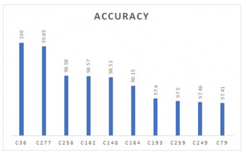
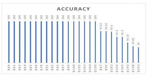
Accuracy is the measurement utilised to decide the best among the selected classifier. Based on the accuracy as shown in Figure 5, KNN (K=1) classifier using Statlog HD dataset (A27) having 100% as the highest accuracy [14] is concluded to be most efficient. Succeeding to the KNN (K=1) classifier, Deep Trained Neocognitron Neural Network (DTNNN) using Cleveland HD dataset (A6) regarded as the next high yielding classifier with 99.85% accuracy [21]. Followed by back-propagation (20 Neurons) using Cleveland HD dataset (A6) having 98.58% accuracy [39] and so on.
Figure 5. Accuracy of top 10 classifiers
Sensitivity is the criteria that is used to examine the impact of each feature on classifier. From Figure 6, on comparing sensitivity of different classifiers, it is observed that Support Vector Machine (SVM) using Cleveland HD dataset (A1) [14] is the finest classifier with 100% sensitivity along with the SVM classifier, Quadratic Discriminant Analysis (QDA) using SPECTF dataset (A25) [37] having the same sensitivity of 100%. Followed by Random Forest using Cleveland HD dataset (A1) having 98.8% sensitivity [22] and so on.
Figure 6. Sensitivity of top 10 classifiers
Specificity is the extent to which a diagnostic test is specific for a particular condition, trait, etc. Based on the Specificity, KNN classifier using SPECT dataset (A8) having 98.11% as the highest Specificity [36] is concluded to be most efficient. Succeeding to the KNN classifier, C4.5 using CDS dataset (A36) regarded as the next high yielding classifier with 97.6% Specificity [36]. Followed by Deep Neural Network (DNN) using Cleveland HD dataset (A24) having 97.5% Specificity [24] is shown in Figure 7, and so on.
Precision is the quality of being exact. Based on the Precision, BNN (3 neurons) [15] using Cleveland HD dataset (A6) having 100% as the highest Precision is concluded to be most efficient. Succeeding to the BNN (3 neurons) Classifier, Deep Trained Neocognitron Neural Network (DTNNN) using Cleveland HD dataset (A6) regarded as the next high yielding classifier with 99.83% Precision [21]. Followed by Genetic Algorithm Optimization of a Convolutional Neural Network (GA-CNN) using Cleveland HD dataset (A6) having 98.34% Precision [5] is shown in Figure 8, and so on.
Figure 7. Specificity of top 10 classifiers
Figure 8. Precision of top 10 classifiers
Figure 9. Auroc of top 10 classifiers
At various threshold levels, the AUROC curve is a performance measurement for classification issues. Based on the AUROC, Ensemble Classifier using Z-Alizadeh Sani CHD dataset (A37) having 95.3% as the highest AUROC [7] is concluded to be most efficient. Succeeding to the Ensemble Classifier, boosted tree using HD dataset (A33) regarded as the next high yielding classifier with 94.5% AUROC [25]. Followed by Binary discriminant using HD dataset (A33) having 93.1% AUROC [24] is shown in Figure 9, and so on.
The F1-measure combines precision and recall into a single measure that captures both attributes while giving them equal importance. Based on the F1-measure, boosted tree Classifier using HD dataset (A33) having 98.2% as the highest F1-measure [25] is concluded to be most efficient. Succeeding to the Deep Neural Network (DNN) Classifier, boosted tree using Cleveland HD dataset (A24) regarded as the next high yielding classifier with 98% F1-measure [24] along with it, Support Vector Machine (SVM) using Cleveland HD dataset (A24) having 98% F1-measure [37] is shown in Figure 10, and so on.
Figure 10. F1-Measure of top 10 classifiers
Data preprocessing is a data mining approach for converting unstructured data into a suitable format. Real-world data is frequently partial, inconsistent, and/or lacking in specific behaviours or trends, as well as including numerous errors [7]. Data preprocessing is a data mining technique used to convert raw data into a useful and efficient format. The steps involved in data preprocessing are Data Cleaning (D.C), Data Transformation (D.T) and Data Reduction (D.R). Data Cleaning involves handling of missing data and noisy data. Missing data can be handled by Ignore the tuples or Fill the Missing values. Noisy data can be handled by Binning Method or Regression or by using Clustering. Data Transformation involves Normalization, Attribute Construction, Discretization, Generalisation, Integration, Manipulation, Normalisation and Smoothing. Data Reduction involves Data Cube Aggregation, Attribute Selection (or) Feature Selection (F.S), Numerosity Reduction, Dimensionality Reduction (or) Feature Extraction (F.E) [57].
In case of HD prediction, the data preprocessing techniques used are Accuracy Based Weighted Aging Classifier Ensemble (AB-WAE), Adaptive-Weighted-Fuzzy-System-Ensemble (AWFSE), Analysis Of Variance (ANOVA), ANN-Fuzzy-AHP (AFP), Ant Colony Optimization (ACO), Ant Colony Optimization Neural Networks (ACONN), Bacterial Foraging Optimization (BFO), Binary Particle Swarm Optimization (BPSO), Binary Particle Swarm Optimization And Rough Sets Based Attribute Reduction (BPSORS-AR), Bootstrap Aggregation (Bagging) With Multi-Objective Optimized Weighted Vote (Bagmoov), CFS (Correlation Based Feature Selection), Chaos Firefly Algorithm And Rough Sets Based Attribute Reduction (CFARS-AR), Chi-Squared (CS), Chi-With-In-Sum-Of-Squares (WSS), Clinical Decision Support System (CDSS), Conditional Mutual Information Maximization (CMIM), Correlation Feature Subset (CFS), Density-Based Spatial Clustering Of Applications With Noise (DBSCAN), Effective HD Prediction System (EHDPS), Ensemble Algorithm Based On Multiple Feature Selection (EA-MFS), Exponentiated Estimate Of The Coefficient Exp(B), Factor Analysis Of Mixed Data (FAMD), Fast Conditional Mutual Information (FCMIM), Fast Correlation-Based Filter (FCBF), Feature Selection (FS), Forward Sequential Search (FSS), Fruit Fly Optimization (FFO), Fuzzy Logic-Based Clinical Decision Support System (FLBCDSS), Gain Ratio (GR), Half Selection(HS), HD Clinical Decision Support System (HDCDSS), Hybrid Ant Colony Optimization Approach (HACO), Hybrid Genetic Algorithm With A New Local Search Algorithm (HGLSA), Hybrid Particle Swarm Optimization With Wrapper Filter (HPSOWF), Information Gain (IG), Instance Based Learner (Ibk), Kernel F-Score Feature Selection (KFFS), Learning Vector Quantization (LVQ), Least Square Twin Support Vector Machine (LSTSVM), Least-Absolute-Shrinkage-Selection-Operator (LASSO), Leave-One-Subject-Out Cross-Validation (LOSO), Local-Learning-Based Features- Selection (LLBFS), Local-Learning-Based-Features-Selection (LLBFS), Mean Fisher Score Feature Selection Algorithm (MFSFSA), Mean Selection(MS), Minimum Redundancy Maximum Relevance (mRMR), Mutual Information-Based Feature Selection (MIFS), Neural Network For Threshold Selection (NNTS), Normalized Mutual Information Feature Selection (NMIFS), Particle Swarm Optimization (PSO), Principal Component Analysis (PCA), Relief-F (RF), Rough Set Based Attribute Reduction (RSBAR), Rough Sets-Based Attributes Selection And Backpropagation Neural Network (RS-BPNN), Standard Scalar (SS), Symmetrical Uncertainty (SU), Synthetic Minority Over-Sampling Technique-Edited Nearest Neighbor (SMOTE-ENN), Weighted Aging Classifier Ensemble (WAE). From the Table 3 it is clear that, most of the data preprocessing techniques used are related to data reduction specifically feature selection.
This section examines the performance parameters of each classifier in combination with various data preprocessing approaches in order to determine the optimum combinations for HD prediction and classification. Table 3 shows the performance measure values of several classifiers with data preparation/preprocessing. A vast number of combinations were investigated, as can be seen in Table 3.
Table 3. Performance metric values of classifier with data preprocessing
|
CWD Code |
Year |
Dataset |
Classifier with Data pre-processing (CWD) |
Number of features used |
Accuracy |
Sensitivity |
Specificity |
Precision |
AUROC |
F1-measure |
Ref |
|
D1 |
2007 |
A6 |
Chi-WSS (F.S)+NB |
4 |
84.48 |
- |
- |
- |
88.46 |
- |
[10] |
|
D2 |
2007 |
A6 |
FSS (F.S)+LR |
8 |
84.81 |
- |
- |
- |
86.43 |
- |
[10] |
|
D3 |
2007 |
A6 |
FSS (F.S)+SVM |
8 |
84.81 |
- |
- |
- |
84.44 |
- |
[10] |
|
D4 |
2007 |
A27 |
Chi-WSS (F.S)+NB |
4 |
84.81 |
- |
- |
- |
87.99 |
- |
[10] |
|
D5 |
2007 |
A27 |
FSS (F.S)+LR |
5 |
85.18 |
- |
- |
- |
86.01 |
- |
[10] |
|
D6 |
2007 |
A27 |
FSS (F.S)+SVM |
4 |
84.44 |
- |
- |
- |
83.92 |
- |
[10] |
|
D7 |
2009 |
A34 |
F-score (F.E)+ ANN |
6 |
77.61 |
77.61 |
88.23 |
- |
82.1 |
- |
[47] |
|
D8 |
2009 |
A34 |
F-score (F.E)+ LS-SVM |
6 |
77.78 |
76.78 |
78.48 |
- |
77.1 |
- |
[47] |
|
D9 |
2009 |
A34 |
Linear kernel F-score (F.E)+ ANN |
13 |
80.74 |
78.95 |
85.5 |
- |
81.1 |
- |
[47] |
|
D10 |
2009 |
A34 |
linear kernel F-score (F.E)+ LS-SVM |
13 |
80 |
86.67 |
76.67 |
- |
78.5 |
- |
[47] |
|
D11 |
2009 |
A34 |
RBF kernel F-score (F.E)+ ANN |
13 |
76.3 |
71.21 |
81.15 |
- |
76.5 |
- |
[47] |
|
D12 |
2009 |
A34 |
RBF kernel F-score (F.E)+ LS-SVM |
13 |
83.7 |
83.92 |
83.54 |
- |
83.1 |
- |
[47] |
|
D13 |
2012 |
A4 |
CFS (F.S)+Bayes theorem (F.S)+ J48 |
3 |
85.18 |
- |
- |
- |
- |
- |
[6] |
|
D14 |
2012 |
A4 |
CFS (F.S)+Bayes theorem (F.S)+ KNN |
3 |
85.55 |
- |
- |
- |
- |
- |
[6] |
|
D15 |
2012 |
A4 |
CFS (F.S)+Bayes theorem (F.S)+ Multi layer perceptron |
3 |
85.18 |
- |
- |
- |
- |
- |
[6] |
|
D16 |
2012 |
A4 |
CFS (F.S)+Bayes theorem (F.S)+ NB |
3 |
80.37 |
- |
- |
- |
- |
- |
[6] |
|
D17 |
2012 |
A4 |
CFS (F.S)+FilteredSubsetEval (F.S)+ KNN |
6 |
80.74 |
- |
- |
- |
- |
- |
[6] |
|
D18 |
2012 |
A4 |
CFS (F.S)+FilteredSubsetEval (F.S)+J48 |
6 |
79.62 |
- |
- |
- |
- |
- |
[6] |
|
D19 |
2012 |
A4 |
CFS (F.S)+FilteredSubsetEval (F.S)+Multi layer Perceptron |
6 |
78.88 |
- |
- |
- |
- |
- |
[6] |
|
D20 |
2012 |
A4 |
CFS (F.S)+FilteredSubsetEval (F.S)+NB |
6 |
85.18 |
- |
- |
- |
- |
- |
[6] |
|
D21 |
2012 |
A4 |
CFS subset eval (F.S)+ Multi layer Perceptron |
7 |
82.22 |
- |
- |
- |
- |
- |
[6] |
|
D22 |
2012 |
A4 |
CFS subset eval (F.S)+J48 |
7 |
81.11 |
- |
- |
- |
- |
- |
[6] |
|
D23 |
2012 |
A4 |
CFS subset eval (F.S)+NB |
7 |
85.5 |
- |
- |
- |
- |
- |
[6] |
|
D24 |
2012 |
A4 |
CFS subset eval(F.S)+KNN |
7 |
78.14 |
- |
- |
- |
- |
- |
[6] |
|
D25 |
2012 |
A4 |
Chi-squared attribute eval (F.S)+ Multi layer Perceptron |
13 |
80.37 |
- |
- |
- |
- |
- |
[6] |
|
D26 |
2012 |
A4 |
Chi-squared attribute eval (F.S)+ J48 |
13 |
76.66 |
- |
- |
- |
- |
- |
[6] |
|
D27 |
2012 |
A4 |
Chi-squared attribute eval (F.S)+ KNN |
13 |
75.18 |
- |
- |
- |
- |
- |
[6] |
|
D28 |
2012 |
A4 |
Chi-squared attribute eval (F.S)+NB |
13 |
83.7 |
- |
- |
- |
- |
- |
[6] |
|
D29 |
2012 |
A4 |
Consistency subset evaluation (F.S) + J48 |
10 |
78.88 |
- |
- |
- |
- |
- |
[6] |
|
D30 |
2012 |
A4 |
Consistency subset evaluation (F.S)+ KNN |
10 |
78.14 |
- |
- |
- |
- |
- |
[6] |
|
D31 |
2012 |
A4 |
Consistency subset evaluation (F.S)+ Multi layer Perceptron |
10 |
81.11 |
- |
- |
- |
- |
- |
[6] |
|
D32 |
2012 |
A4 |
Consistency subset evaluation (F.S)+ NB |
10 |
84.07 |
- |
- |
- |
- |
- |
[6] |
|
D33 |
2012 |
A4 |
Filtered attribute Evaluation (F.S)+ J48 |
13 |
76.66 |
- |
- |
- |
- |
- |
[6] |
|
D34 |
2012 |
A4 |
Filtered attribute Evaluation (F.S)+ KNN |
13 |
75.18 |
- |
- |
- |
- |
- |
[6] |
|
D35 |
2012 |
A4 |
Filtered attribute Evaluation (F.S)+ Multi layer Perceptron |
13 |
80.37 |
- |
- |
- |
- |
- |
[6] |
|
D36 |
2012 |
A4 |
Filtered attribute Evaluation (F.S)+ NB |
13 |
83.7 |
- |
- |
- |
- |
- |
[6] |
|
D37 |
2012 |
A4 |
Filteredsubset eval (F.S)+ J48 |
6 |
79.6 |
- |
- |
- |
- |
- |
[6] |
|
D38 |
2012 |
A4 |
Filteredsubset eval (F.S)+ Multi layer Perceptron |
6 |
78.88 |
- |
- |
- |
- |
- |
[6] |
|
D39 |
2012 |
A4 |
Filteredsubset eval (F.S)+ NB |
6 |
85.18 |
- |
- |
- |
- |
- |
[6] |
|
D40 |
2012 |
A4 |
Gain ratio attribute Evaluation (F.S)+ Multi layer Perceptron |
13 |
78.88 |
- |
- |
- |
- |
- |
[6] |
|
D41 |
2012 |
A4 |
Gain ratio attribute Evaluation (F.S)+ NB |
13 |
83.7 |
- |
- |
- |
- |
- |
[6] |
|
D42 |
2012 |
A4 |
Gain ratio attribute Evaluation (F.S)+ J48 |
13 |
76.66 |
- |
- |
- |
- |
- |
[6] |
|
D43 |
2012 |
A4 |
Gain ratio attribute Evaluation (F.S)+ KNN |
13 |
75.18 |
- |
- |
- |
- |
- |
[6] |
|
D44 |
2012 |
A4 |
Info gain attribute Evaluation (F.S)+ Multi layer Perceptron |
13 |
80.37 |
- |
- |
- |
- |
- |
[6] |
|
D45 |
2012 |
A4 |
Info gain attribute Evaluation (F.S) + J48 |
13 |
76.66 |
- |
- |
- |
- |
- |
[6] |
|
D46 |
2012 |
A4 |
Info gain attribute Evaluation (F.S)+ KNN |
13 |
75.18 |
- |
- |
- |
- |
- |
[6] |
|
D47 |
2012 |
A4 |
Info gain attribute Evaluation (F.S)+ NB |
13 |
83.7 |
- |
- |
- |
- |
- |
[6] |
|
D48 |
2012 |
A4 |
Latent semantic analysis (F.S)+ Multi layer Perceptron |
1 |
52.96 |
- |
- |
- |
- |
- |
[6] |
|
D49 |
2012 |
A4 |
Latent semantic analysis (F.S)+ J48 |
1 |
55.55 |
- |
- |
- |
- |
- |
[6] |
|
D50 |
2012 |
A4 |
Latent semantic analysis (F.S)+ KNN |
1 |
51.11 |
- |
- |
- |
- |
- |
[6] |
|
D51 |
2012 |
A4 |
Latent semantic analysis (F.S)+ NB |
1 |
54.07 |
- |
- |
- |
- |
- |
[6] |
|
D52 |
2012 |
A4 |
One attribute eval (F.S)+ J48 |
13 |
76.66 |
- |
- |
- |
- |
- |
[6] |
|
D53 |
2012 |
A4 |
One attribute eval (F.S)+ KNN |
13 |
75.18 |
- |
- |
- |
- |
- |
[6] |
|
D54 |
2012 |
A4 |
One attribute eval (F.S)+ Multi layer Perceptron |
13 |
79.25 |
- |
- |
- |
- |
- |
[6] |
|
D55 |
2012 |
A4 |
One attribute eval (F.S)+ NB |
13 |
83.7 |
- |
- |
- |
- |
- |
[6] |
|
D56 |
2012 |
A4 |
Relief attribute evaluation (F.S)+ J48 |
13 |
76.66 |
- |
- |
- |
- |
- |
[6] |
|
D57 |
2012 |
A4 |
Relief attribute evaluation (F.S)+ KNN |
13 |
75.18 |
- |
- |
- |
- |
- |
[6] |
|
D58 |
2012 |
A4 |
Relief attribute evaluation (F.S)+ Multi layer Perceptron |
13 |
78.14 |
- |
- |
- |
- |
- |
[6] |
|
D59 |
2012 |
A4 |
Relief attribute evaluation (F.S)+ NB |
13 |
83.7 |
- |
- |
- |
- |
- |
[6] |
|
D60 |
2013 |
A29 |
ANN+PCA (F.E) |
4 |
100 |
- |
- |
- |
- |
- |
[42] |
|
D61 |
2013 |
A29 |
ANN+χ 2 (F.S) |
4 |
100 |
- |
- |
- |
- |
- |
[42] |
|
D62 |
2013 |
A29 |
KNN+SU (F.S+D.T) |
4 |
97.5 |
- |
- |
- |
- |
- |
[42] |
|
D63 |
2013 |
A7 |
ANN+GA (F.S+.D.T) |
5 |
100 |
- |
- |
- |
- |
- |
[42] |
|
D64 |
2013 |
A7 |
ANN+PCA (F.E) |
5 |
100 |
- |
- |
- |
- |
- |
[42] |
|
D65 |
2013 |
A7 |
ANN+χ 2 (F.S) |
5 |
100 |
- |
- |
- |
- |
- |
[42] |
|
D66 |
2013 |
A7 |
KNN+SU (F.S+D.T) |
5 |
100 |
- |
- |
- |
- |
- |
[42] |
|
D67 |
2013 |
A27 |
ANN+GA (F.S+.D.T) |
7 |
99.62 |
- |
- |
- |
- |
- |
[42] |
|
D68 |
2013 |
A27 |
ANN+PCA (F.E) |
7 |
98.14 |
- |
- |
- |
- |
- |
[42] |
|
D69 |
2013 |
A27 |
ANN+χ 2 (F.S) |
7 |
97.7 |
- |
- |
- |
- |
- |
[42] |
|
D70 |
2013 |
A27 |
KNN+SU (F.S+D.T) |
7 |
100 |
- |
- |
- |
- |
- |
[42] |
|
D71 |
2013 |
A28 |
HS (F.S) + RBF |
7 |
83.44 |
84 |
83 |
- |
- |
- |
[41] |
|
D72 |
2013 |
A28 |
MS (F.S) + RBF |
6 |
81.75 |
82 |
82 |
- |
- |
- |
[41] |
|
D73 |
2013 |
A28 |
NNTS (F.S)+ RBF |
3 |
84.46 |
82 |
82 |
- |
- |
- |
[41] |
|
D74 |
2013 |
A28 |
RBF + CMIM (F.S) |
3 |
83.78 |
- |
- |
- |
- |
- |
[41] |
|
D75 |
2013 |
A28 |
RBF + FCBF (F.S) |
4 |
80.74 |
- |
- |
- |
- |
- |
[41] |
|
D76 |
2013 |
A28 |
RBF + Fuzzyentropy-NNTS (F.S) |
4 |
84.46 |
- |
- |
- |
- |
- |
[41] |
|
D77 |
2013 |
A28 |
RBF + IG (F.S) |
5 |
82.43 |
- |
- |
- |
- |
- |
[41] |
|
D78 |
2013 |
A28 |
RBF + MIFS (F.S) |
5 |
76.35 |
- |
- |
- |
- |
- |
[41] |
|
D79 |
2013 |
A28 |
RBF + mRMR (F.S) |
4 |
83.78 |
- |
- |
- |
- |
- |
[41] |
|
D80 |
2013 |
A28 |
RBF + NMIFS (F.S) |
4 |
84.12 |
- |
- |
- |
- |
- |
[41] |
|
D81 |
2013 |
A27 |
HS (F.S) + RBF |
7 |
84.81 |
85 |
84 |
- |
89 |
- |
[41] |
|
D82 |
2013 |
A27 |
MS (F.S) + RBF |
6 |
84.44 |
85 |
84 |
- |
89 |
- |
[41] |
|
D83 |
2013 |
A27 |
NNTS (F.S)+ RBF |
4 |
85.19 |
85 |
86 |
- |
89 |
- |
[41] |
|
D84 |
2013 |
A27 |
RBF + CMIM (F.S) |
3 |
83.33 |
- |
- |
- |
- |
- |
[41] |
|
D85 |
2013 |
A27 |
RBF + FCBF (F.S) |
4 |
82.96 |
- |
- |
- |
- |
- |
[41] |
|
D86 |
2013 |
A27 |
RBF + Fuzzyentropy-NNTS (F.S) |
4 |
85.18 |
- |
- |
- |
- |
- |
[41] |
|
D87 |
2013 |
A27 |
RBF + IG (F.S) |
5 |
84.81 |
- |
- |
- |
- |
- |
[41] |
|
D88 |
2013 |
A27 |
RBF + MIFS (F.S) |
5 |
83.7 |
- |
- |
- |
- |
- |
[41] |
|
D89 |
2013 |
A27 |
RBF + mRMR (F.S) |
4 |
84.44 |
- |
- |
- |
- |
- |
[41] |
|
D90 |
2013 |
A27 |
RBF + NMIFS (F.S) |
4 |
84.81 |
- |
- |
- |
- |
- |
[41] |
|
D91 |
2013 |
A30 |
Chi square (F.S) + ANN |
5 |
100 |
- |
- |
- |
- |
- |
[39] |
|
D92 |
2013 |
A30 |
GA(F.S+.D.T)+ ANN |
5 |
100 |
- |
- |
- |
- |
- |
[39] |
|
D93 |
2013 |
A30 |
PCA (F.E)+ ANN |
5 |
100 |
- |
- |
- |
- |
- |
[39] |
|
D94 |
2013 |
A2 |
Chi square (F.S) + ANN |
5 |
97.7 |
- |
- |
- |
- |
- |
[39] |
|
D95 |
2013 |
A2 |
GA(F.S+.D.T)+ ANN |
5 |
99.62 |
- |
- |
- |
- |
- |
[39] |
|
D96 |
2013 |
A2 |
PCA (F.E) + ANN |
5 |
98.14 |
- |
- |
- |
- |
- |
[39] |
|
D97 |
2013 |
A30 |
GA(F.S+.D.T)+ANN |
12 |
100 |
- |
- |
- |
- |
- |
[43] |
|
D98 |
2013 |
A30 |
KNN (K=1) |
12 |
95 |
- |
- |
- |
- |
- |
[43] |
|
D99 |
2013 |
A30 |
KNN+GA (F.S+.D.T) |
12 |
100 |
- |
- |
- |
- |
- |
[43] |
|
D100 |
2013 |
A30 |
NN+PCA (F.E) |
12 |
100 |
- |
- |
- |
- |
- |
[43] |
|
D101 |
2013 |
A30 |
NN+χ 2 (F.S) |
2 |
100 |
- |
- |
- |
- |
- |
[43] |
|
D102 |
2013 |
A27 |
GA(F.S+.D.T)+ANN |
13 |
99.6 |
- |
- |
- |
- |
- |
[43] |
|
D103 |
2013 |
A27 |
KNN (K=1) |
13 |
100 |
- |
- |
- |
- |
- |
[43] |
|
D104 |
2013 |
A27 |
KNN+GA (F.S+.D.T) |
13 |
100 |
- |
- |
- |
- |
- |
[43] |
|
D105 |
2013 |
A27 |
NN+PCA (F.E) |
13 |
98.14 |
- |
- |
- |
- |
- |
[43] |
|
D106 |
2013 |
A27 |
NN+χ 2 (F.S) |
13 |
97.7 |
- |
- |
- |
- |
- |
[43] |
|
D107 |
2015 |
A6 |
GA (F.S+.D.T)+ Naïve Bayes |
8 |
84.16 |
- |
- |
- |
- |
- |
[21] |
|
D108 |
2015 |
A6 |
GA(F.S+.D.T) + J48 |
8 |
77.56 |
- |
- |
- |
- |
- |
[21] |
|
D109 |
2015 |
A6 |
GA(F.S+.D.T) + RBF |
8 |
85.48 |
- |
- |
- |
- |
- |
[21] |
|
D110 |
2017 |
A6 |
BPSO(F.S+D.T) + RSBAR (F.S) + SVM |
9 |
75.9 |
- |
- |
- |
- |
- |
[30] |
|
D111 |
2017 |
A6 |
BPSO(F.S+D.T) + RSBAR (F.S) + Naive Bayes |
9 |
79.6 |
- |
- |
- |
- |
- |
[30] |
|
D112 |
2017 |
A6 |
CF + RSBAR (F.S)+ ANN |
9 |
81.5 |
- |
- |
- |
- |
- |
[30] |
|
D113 |
2017 |
A6 |
modified DE (F.S) + fuzzy AHP + feed-forward NN |
9 |
83 |
- |
- |
- |
- |
- |
[30] |
|
D114 |
2017 |
A37 |
Adaboost + ANOVA F(F.S) |
29 |
90.11 |
- |
- |
- |
- |
91.35 |
[49] |
|
D115 |
2017 |
A37 |
Adaboost + CHI(F.S) |
34 |
91.21 |
- |
- |
- |
- |
93.22 |
[49] |
|
D116 |
2017 |
A37 |
Adaboost + LR.coef (F.S)(Embedded+SVM) |
12 |
89.01 |
- |
- |
- |
- |
89.74 |
[49] |
|
D117 |
2017 |
A37 |
Adaboost + MutualInfo (F.S) |
10 |
90.01 |
- |
- |
- |
- |
91.02 |
[49] |
|
D118 |
2017 |
A37 |
Adaboost + RF.coef (F.S) (Embedded+SVM) |
28 |
89.01 |
- |
- |
- |
- |
89.74 |
[49] |
|
D119 |
2017 |
A37 |
Adaboost + SVM.coef (F.S)(Embedded+SVM) |
16 |
90.11 |
- |
- |
- |
- |
91.07 |
[49] |
|
D120 |
2017 |
A37 |
GBDT + ANOVA F(F.S) (Filter+Adaboost) |
29 |
86.81 |
- |
- |
- |
- |
90.1 |
[49] |
|
D121 |
2017 |
A37 |
GBDT + CHI (F.S) (Filter+Adaboost) |
34 |
86.81 |
- |
- |
- |
- |
87.05 |
[49] |
|
D122 |
2017 |
A37 |
GBDT + LR.coef (F.S) (Embedded+SVM) |
12 |
84.62 |
- |
- |
- |
- |
88.18 |
[49] |
|
D123 |
2017 |
A37 |
GBDT + MutualInfo (F.S) (Filter+Adaboost) |
10 |
83.52 |
- |
- |
- |
- |
88.3 |
[49] |
|
D124 |
2017 |
A37 |
GBDT + RF.coef (F.S)(Embedded+SVM) |
28 |
86.81 |
- |
- |
- |
- |
90.1 |
[49] |
|
D125 |
2017 |
A37 |
GBDT + SVM.coef (F.S) (Embedded+SVM) |
16 |
83.52 |
- |
- |
- |
- |
85.37 |
[49] |
|
D126 |
2017 |
A37 |
KNN + ANOVA F (F.S)(Filter+Adaboost) |
29 |
85.71 |
- |
- |
- |
- |
88.03 |
[49] |
|
D127 |
2017 |
A37 |
KNN + CHI (F.S)(Filter+Adaboost) |
34 |
89.01 |
- |
- |
- |
- |
85.83 |
[49] |
|
D128 |
2017 |
A37 |
KNN + LR.coef (F.S)(Embedded+SVM) |
12 |
85.71 |
- |
- |
- |
- |
88.18 |
[49] |
|
D129 |
2017 |
A37 |
KNN + MutualInfo (F.S) (Filter+Adaboost) |
10 |
86.81 |
- |
- |
- |
- |
87.84 |
[49] |
|
D130 |
2017 |
A37 |
KNN + RF.coef (F.S)(Embedded+SVM) |
28 |
85.71 |
- |
- |
- |
- |
88.03 |
[49] |
|
D131 |
2017 |
A37 |
KNN + SVM.coef (F.S) (Embedded+SVM) |
16 |
89.01 |
- |
- |
- |
- |
90.51 |
[49] |
|
D132 |
2017 |
A37 |
LR + ANOVA F (F.S)(Filter+Adaboost) |
29 |
89.01 |
- |
- |
- |
- |
90.51 |
[49] |
|
D133 |
2017 |
A37 |
LR + CHI (F.S)(Filter+Adaboost) |
34 |
87.91 |
- |
- |
- |
- |
89.18 |
[49] |
|
D134 |
2017 |
A37 |
LR + LR.coef (F.S)(Embedded+SVM) |
12 |
91.21 |
- |
- |
- |
- |
90.84 |
[49] |
|
D135 |
2017 |
A37 |
LR + MutualInfo (F.S) (Filter+Adaboost) |
10 |
89.01 |
- |
- |
- |
- |
89.74 |
[49] |
|
D136 |
2017 |
A37 |
LR + RF.coef (F.S)(Embedded+SVM) |
28 |
89.01 |
- |
- |
- |
- |
90.51 |
[49] |
|
D137 |
2017 |
A37 |
LR + SVM.coef (F.S)(Embedded+SVM) |
16 |
92.31 |
- |
- |
- |
- |
92.18 |
[49] |
|
D138 |
2017 |
A37 |
MLP + ANOVA F(F.S) (Filter+Adaboost) |
29 |
90.11 |
- |
- |
- |
- |
91.07 |
[49] |
|
D139 |
2017 |
A37 |
MLP + CHI(F.S) (Filter+Adaboost) |
34 |
90.11 |
- |
- |
- |
- |
89.51 |
[49] |
|
D140 |
2017 |
A37 |
MLP + LR.coef(F.S) (Embedded+SVM) |
12 |
90.11 |
- |
- |
- |
- |
91.07 |
[49] |
|
D141 |
2017 |
A37 |
MLP + MutualInfo(F.S) (Filter+Adaboost) |
10 |
85.71 |
- |
- |
- |
- |
88.77 |
[49] |
|
D142 |
2017 |
A37 |
MLP + RF.coef (F.S)(Embedded+SVM) |
28 |
89.01 |
- |
- |
- |
- |
89.74 |
[49] |
|
D143 |
2017 |
A37 |
MLP + SVM.coef (F.S)(Embedded+SVM) |
16 |
91.21 |
- |
- |
- |
- |
91.63 |
[49] |
|
D144 |
2017 |
A37 |
RF + RF.coef (F.S)(Embedded+SVM) |
28 |
85.71 |
- |
- |
- |
- |
90.22 |
[49] |
|
D145 |
2017 |
A37 |
RF + SVM.coef (F.S)(Embedded+SVM) |
16 |
87.91 |
- |
- |
- |
- |
89.18 |
[49] |
|
D146 |
2017 |
A37 |
RF + ANOVA F (F.S) (Filter+Adaboost) |
29 |
86.81 |
- |
- |
- |
- |
90.1 |
[49] |
|
D147 |
2017 |
A37 |
RF + CHI (F.S)(Filter+Adaboost) |
34 |
85.52 |
- |
- |
- |
- |
85.84 |
[49] |
|
D148 |
2017 |
A37 |
RF + LR.coef (F.S)(Embedded+SVM) |
12 |
86.81 |
- |
- |
- |
- |
88.61 |
[49] |
|
D149 |
2017 |
A37 |
RF + MutualInfo(F.S) (Filter+Adaboost) |
10 |
87.91 |
- |
- |
- |
- |
89.18 |
[49] |
|
D150 |
2017 |
A37 |
SVM + RF.coef (F.S)(Embedded+SVM) |
28 |
90.11 |
- |
- |
- |
- |
91.07 |
[49] |
|
D151 |
2017 |
A37 |
SVM + ANOVA F (F.S)(Filter+Adaboost) |
29 |
86.81 |
- |
- |
- |
- |
89.36 |
[49] |
|
D152 |
2017 |
A37 |
SVM + CHI (F.S) (Filter+Adaboost) |
34 |
87.91 |
- |
- |
- |
- |
89.94 |
[49] |
|
D153 |
2017 |
A37 |
SVM + LR.coef (F.S) (Embedded+SVM) |
12 |
90.11 |
- |
- |
- |
- |
91.07 |
[49] |
|
D154 |
2017 |
A37 |
SVM + MutualInfo (F.S)(Filter+Adaboost) |
10 |
89.01 |
- |
- |
- |
- |
90.51 |
[49] |
|
D155 |
2017 |
A37 |
SVM + SVM.coef (F.S)(Embedded+SVM) |
16 |
91.21 |
- |
- |
- |
- |
91.63 |
[49] |
|
D156 |
2018 |
A27 |
Decision Tree + Gain Ratio (F.S) |
9 |
84.1 |
- |
- |
- |
- |
- |
[32] |
|
D157 |
2018 |
A27 |
Neural Network with Fuzzy |
9 |
80 |
- |
- |
- |
- |
- |
[32] |
|
D158 |
2018 |
A27 |
Neural Network with Genetic Algorithm (F.S+.D.T) |
9 |
80.99 |
- |
- |
- |
- |
- |
[32] |
|
D159 |
2018 |
A27 |
Support Vector Machine |
13 |
82.22 |
- |
- |
- |
- |
- |
[32] |
|
D160 |
2018 |
A27 |
Vote + Naïve Bayes and Logistic Regression (F.S) |
9 |
87.41 |
- |
- |
- |
- |
- |
[32] |
|
D161 |
2018 |
A27 |
Vote + Naïve Bayes and Logistic Regression (F.S) |
9 |
87.41 |
- |
- |
- |
- |
- |
[32] |
|
D162 |
2020 |
A6 |
CFS (F.S)+ PSO (F.S)+K-means (D.T)+ MLP |
13 |
90.28 |
- |
- |
- |
- |
- |
[20] |
|
D163 |
2020 |
A6 |
DBSCAN + SMOTE-ENN (D.B- D.T)+ XGBOOST |
8 |
98.4 |
- |
- |
- |
- |
- |
[20] |
|
D164 |
2020 |
A6 |
FAMD (F.S)+ RF |
13 |
93.44 |
- |
- |
- |
- |
- |
[20] |
|
D165 |
2020 |
A6 |
HDPM |
13 |
98.4 |
- |
- |
98.57 |
- |
- |
[20] |
|
D166 |
2020 |
A6 |
Majority Vote with NB, BN, RF and MP |
13 |
85.48 |
- |
- |
- |
- |
- |
[20] |
|
D167 |
2020 |
A6 |
MFSFSA (F.S)+ SVM |
13 |
81.19 |
- |
- |
- |
- |
- |
[20] |
|
D168 |
2020 |
A6 |
Relief (F.S) +LR |
13 |
89 |
- |
- |
- |
- |
- |
[20] |
|
D169 |
2020 |
A27 |
CFARS-AR (F.S) |
13 |
88.3 |
- |
- |
- |
- |
- |
[20] |
|
D170 |
2020 |
A27 |
DBSCAN + SMOTE-ENN (D.B- D.T)+ XGBOOST |
9 |
95.9 |
- |
- |
- |
- |
- |
[20] |
|
D171 |
2020 |
A27 |
HDPM |
13 |
95.9 |
- |
- |
97.14 |
- |
- |
[20] |
|
D172 |
2020 |
A27 |
RS-BPNN (F.S) |
13 |
90.4 |
- |
- |
- |
- |
- |
[20] |
|
D173 |
2020 |
A27 |
Vote with NB and LR (F.S) |
13 |
87.41 |
- |
- |
- |
- |
- |
[20] |
|
D174 |
2020 |
A6 |
FAMD (F.S) + DT |
13 |
81.96 |
71.42 |
90.9 |
- |
81.16 |
78.43 |
[32] |
|
D175 |
2020 |
A6 |
FAMD (F.S)+ KNN |
13 |
90.16 |
92.85 |
87.87 |
- |
90.36 |
89.65 |
[5] |
|
D176 |
2020 |
A6 |
FAMD (F.S)+ LR |
13 |
91.8 |
92.85 |
90.9 |
- |
91.88 |
91.22 |
[5] |
|
D177 |
2020 |
A6 |
FAMD (F.S)+ RF |
13 |
93.44 |
89.28 |
96.96 |
- |
93.12 |
92.59 |
[5] |
|
D178 |
2020 |
A6 |
FAMD (F.S)+ SVM |
13 |
91.8 |
100 |
84.84 |
- |
92.42 |
91.8 |
[5] |
|
D179 |
2020 |
A6 |
L1 Linear SVM + L2 Linear SVM & RBF SVM |
13 |
92.22 |
82.92 |
100 |
- |
- |
- |
[5] |
|
D180 |
2020 |
A6 |
LASSO (F.S)+ SVM |
13 |
88 |
75 |
96 |
- |
- |
- |
[5] |
|
D181 |
2020 |
A6 |
mRMR (F.S)+ NB |
13 |
84 |
77 |
90 |
- |
- |
- |
[5] |
|
D182 |
2020 |
A6 |
PSO (F.S) + SVM |
13 |
84.36 |
- |
- |
- |
- |
- |
[5] |
|
D183 |
2020 |
A6 |
RBF kernal - based SVM |
13 |
81.19 |
72.92 |
88.68 |
- |
- |
- |
[5] |
|
D184 |
2020 |
A6 |
Relief (F.S)+ LR |
13 |
89 |
77 |
98 |
- |
- |
- |
[5] |
|
D185 |
2020 |
A1 |
ANN - FUZZY- AHP |
13 |
91.1 |
- |
- |
- |
- |
- |
[18] |
|
D186 |
2020 |
A1 |
ANN+Fuzzy Logic |
13 |
87.4 |
- |
- |
- |
- |
- |
[18] |
|
D187 |
2020 |
A1 |
FCMIM (DISC) + ANN |
6 |
75.23 |
- |
- |
- |
- |
- |
[18] |
|
D188 |
2020 |
A1 |
FCMIM (DISC) + DT |
6 |
79.12 |
- |
- |
- |
- |
- |
[18] |
|
D189 |
2020 |
A1 |
FCMIM (DISC) + KNN |
6 |
82.11 |
- |
- |
- |
- |
- |
[18] |
|
D190 |
2020 |
A1 |
FCMIM (DISC) + LR |
6 |
88.67 |
- |
- |
- |
- |
- |
[18] |
|
D191 |
2020 |
A1 |
FCMIM (DISC)+ NB |
6 |
86.01 |
- |
- |
- |
- |
- |
[18] |
|
D192 |
2020 |
A1 |
FCMIM (DISC)+ SVM(Linear) |
6 |
92.37 |
- |
- |
- |
- |
- |
[18] |
|
D193 |
2020 |
A1 |
LASSO (F.S) + ANN |
6 |
79 |
- |
- |
- |
- |
- |
[18] |
|
D194 |
2020 |
A1 |
LASSO (F.S)+ DT |
6 |
78 |
- |
- |
- |
- |
- |
[18] |
|
D195 |
2020 |
A1 |
LASSO (F.S)+ KNN |
6 |
79 |
- |
- |
- |
- |
- |
[18] |
|
D196 |
2020 |
A1 |
LASSO (F.S)+ LR |
6 |
85 |
- |
- |
- |
- |
- |
[18] |
|
D197 |
2020 |
A1 |
LASSO (F.S)+ NB |
6 |
79 |
- |
- |
- |
- |
- |
[18] |
|
D198 |
2020 |
A1 |
LASSO(F.S) + SVM(Linear) |
6 |
86 |
- |
- |
- |
- |
- |
[18] |
|
D199 |
2020 |
A1 |
LASSO(F.S) + SVM(RBF) |
6 |
85 |
- |
- |
- |
- |
- |
[18] |
|
D200 |
2020 |
A1 |
LLBFS (F.S) + SVM (Linear) |
6 |
87 |
- |
- |
- |
- |
- |
[18] |
|
D201 |
2020 |
A1 |
LLBFS (F.S)+ ANN |
6 |
80 |
- |
- |
- |
- |
- |
[18] |
|
D202 |
2020 |
A1 |
LLBFS (F.S)+ DT |
6 |
74 |
- |
- |
- |
- |
- |
[18] |
|
D203 |
2020 |
A1 |
LLBFS (F.S)+ KNN |
6 |
77 |
- |
- |
- |
- |
- |
[18] |
|
D204 |
2020 |
A1 |
LLBFS (F.S)+ LR |
6 |
88 |
- |
- |
- |
- |
- |
[18] |
|
D205 |
2020 |
A1 |
LLBFS (F.S)+ NB |
6 |
76 |
- |
- |
- |
- |
- |
[18] |
|
D206 |
2020 |
A1 |
LLBFS (F.S)+ SVM(RBF) |
6 |
82 |
- |
- |
- |
- |
- |
[18] |
|
D207 |
2020 |
A1 |
MLP + SVM |
13 |
80.41 |
- |
- |
- |
- |
- |
[18] |
|
D208 |
2020 |
A1 |
mRMR (F.S) + ANN |
6 |
78 |
- |
- |
- |
- |
- |
[18] |
|
D209 |
2020 |
A1 |
mRMR (F.S) + DT |
6 |
78 |
- |
- |
- |
- |
- |
[18] |
|
D210 |
2020 |
A1 |
mRMR (F.S) + KNN |
6 |
78 |
- |
- |
- |
- |
- |
[18] |
|
D211 |
2020 |
A1 |
mRMR (F.S) + LR |
6 |
83 |
- |
- |
- |
- |
- |
[18] |
|
D212 |
2020 |
A1 |
mRMR (F.S) + SVM(RBF) |
6 |
83 |
- |
- |
- |
- |
- |
[18] |
|
D213 |
2020 |
A1 |
mRMR (F.S)+ NB |
6 |
77 |
- |
- |
- |
- |
- |
[18] |
|
D214 |
2020 |
A1 |
mRMR (F.S)+ SVM(Linear) |
6 |
87 |
- |
- |
- |
- |
- |
[18] |
|
D215 |
2020 |
A1 |
Relief (F.S)+ ANN |
6 |
75 |
- |
- |
- |
- |
- |
[18] |
|
D216 |
2020 |
A1 |
Relief (F.S)+ DT |
6 |
73 |
- |
- |
- |
- |
- |
[18] |
|
D217 |
2020 |
A1 |
Relief (F.S)+ KNN |
6 |
74 |
- |
- |
- |
- |
- |
[18] |
|
D218 |
2020 |
A1 |
Relief (F.S)+ LR |
6 |
85 |
- |
- |
- |
- |
- |
[18] |
|
D219 |
2020 |
A1 |
Relief (F.S)+ NB |
6 |
76 |
- |
- |
- |
- |
- |
[18] |
|
D220 |
2020 |
A1 |
Relief (F.S)+ SVM(Linear) |
6 |
86 |
- |
- |
- |
- |
- |
[18] |
|
D221 |
2020 |
A1 |
Relief (F.S)+ SVM(RBF) |
6 |
81 |
- |
- |
- |
- |
- |
[18] |
|
D222 |
2020 |
A1 |
Three phase technique based on ANN |
13 |
88.89 |
- |
- |
- |
- |
- |
[18] |
|
D223 |
2020 |
A6 |
ABBM + LASSO (F.S) |
8 |
90.75 |
- |
- |
- |
- |
- |
[26] |
|
D224 |
2020 |
A6 |
ABBM + Relief (F.S) |
7 |
95.38 |
- |
- |
- |
- |
- |
[26] |
|
D225 |
2020 |
A6 |
Adaboost + LASSO (F.S) |
8 |
90.75 |
- |
- |
- |
- |
- |
[26] |
|
D226 |
2020 |
A6 |
Adaboost + Relief (F.S) |
7 |
92.85 |
- |
- |
- |
- |
- |
[26] |
|
D227 |
2020 |
A6 |
DT + LASSO (F.S) |
13 |
88.6 |
- |
- |
- |
- |
- |
[26] |
|
D228 |
2020 |
A6 |
DT + Relief (F.S) |
13 |
89.12 |
- |
- |
- |
- |
- |
[26] |
|
D229 |
2020 |
A6 |
GBBM + LASSO (F.S) |
8 |
97.85 |
- |
- |
- |
- |
- |
[26] |
|
D230 |
2020 |
A6 |
GBBM + Relief (F.S) |
7 |
98.32 |
- |
- |
- |
- |
- |
[26] |
|
D231 |
2020 |
A6 |
KNN + LASSO (F.S) |
13 |
93 |
- |
- |
- |
- |
- |
[26] |
|
D232 |
2020 |
A6 |
KNN + LASSO (F.S) |
8 |
93 |
- |
- |
- |
- |
- |
[26] |
|
D233 |
2020 |
A6 |
KNN + Relief (F.S) |
13 |
94.11 |
- |
- |
- |
- |
- |
[26] |
|
D234 |
2020 |
A6 |
KNN + Relief (F.S) |
7 |
94.11 |
- |
- |
- |
- |
- |
[26] |
|
D235 |
2020 |
A6 |
KNNBM + LASSO (F.S) |
13 |
96.6 |
- |
- |
- |
- |
- |
[26] |
|
D236 |
2020 |
A6 |
KNNBM + LASSO (F.S) |
8 |
96.6 |
- |
- |
- |
- |
- |
[26] |
|
D237 |
2020 |
A6 |
KNNBM + Relief (F.S) |
13 |
90.75 |
- |
- |
- |
- |
- |
[26] |
|
D238 |
2020 |
A6 |
KNNBM + Relief (F.S) |
7 |
98.05 |
- |
- |
- |
- |
- |
[26] |
|
D239 |
2020 |
A6 |
RFBM + LASSO (F.S) |
8 |
97.65 |
- |
- |
- |
- |
- |
[26] |
|
D240 |
2020 |
A6 |
RFBM + Relief (F.S) |
7 |
99.05 |
- |
- |
- |
- |
- |
[26] |
|
2020 |
A20 |
RFBM + LASSO (F.S) |
13 |
97.65 |
- |
- |
- |
- |
- |
[26] |
|
|
D242 |
2020 |
A20 |
RFBM + Relief (F.S) |
13 |
96.6 |
- |
- |
- |
- |
- |
[26] |
|
D243 |
2020 |
A21 |
GB + LASSO (F.S) |
13 |
92.85 |
- |
- |
- |
- |
- |
[26] |
|
D244 |
2020 |
A21 |
GB + Relief (F.S) |
13 |
88.65 |
- |
- |
- |
- |
- |
[26] |
|
D245 |
2020 |
A21 |
RF + LASSO (F.S) |
13 |
86.97 |
- |
- |
- |
- |
- |
[26] |
|
D246 |
2020 |
A21 |
RF + Relief (F.S) |
13 |
97.89 |
- |
- |
- |
- |
- |
[26] |
|
2020 |
A18 |
GBBM + LASSO (F.S) |
13 |
97.85 |
- |
- |
- |
- |
- |
[26] |
|
|
D248 |
2020 |
A18 |
GBBM + Relief (F.S) |
13 |
98.32 |
- |
- |
- |
- |
- |
[26] |
|
D249 |
2020 |
A16 |
DTBM + LASSO (F.S) |
8 |
88.65 |
- |
- |
- |
- |
- |
[26] |
|
D250 |
2020 |
A16 |
DTBM + Relief (F.S) |
7 |
90.22 |
- |
- |
- |
- |
- |
[26] |
|
D251 |
2020 |
A17 |
Adaboost + LASSO (F.S) |
16 |
90.75 |
- |
- |
- |
- |
- |
[26] |
|
D252 |
2020 |
A17 |
Adaboost + Relief (F.S) |
16 |
92.85 |
- |
- |
- |
- |
- |
[26] |
|
D253 |
2020 |
A47 |
DTBM + LASSO (F.S) |
13 |
88.65 |
- |
- |
- |
- |
- |
[26] |
|
D254 |
2020 |
A47 |
DTBM + Relief (F.S) |
13 |
97.65 |
- |
- |
- |
- |
- |
[26] |
|
D255 |
2020 |
A40 |
ABBM + LASSO (F.S) |
13 |
90.75 |
- |
- |
- |
- |
- |
[26] |
|
D256 |
2020 |
A27 |
ABBM + Relief (F.S) |
13 |
97.85 |
- |
- |
- |
- |
- |
[26] |
|
D257 |
2020 |
A27 |
GB + LASSO (F.S) |
8 |
92.85 |
- |
- |
- |
- |
- |
[26] |
|
D258 |
2020 |
A27 |
GB + Relief (F.S) |
7 |
96.22 |
- |
- |
- |
- |
- |
[26] |
|
D259 |
2011 |
A16 |
FLBCDSS |
13 |
79.5 |
80 |
59.09 |
- |
- |
- |
[35] |
|
D260 |
2011 |
A15 |
FLBCDSS |
13 |
56.47 |
62.5 |
53.76 |
- |
- |
- |
[35] |
|
D261 |
2011 |
A13 |
FLBCDSS |
13 |
55.99 |
72.47 |
30.58 |
- |
- |
- |
[35] |
|
D262 |
2013 |
A1 |
FFNN + EXP(B) |
8 |
85.2 |
- |
- |
- |
- |
- |
[8] |
|
D263 |
2013 |
A1 |
FFNN + PCA (F.E) |
8 |
87.6 |
- |
- |
- |
- |
- |
[8] |
|
D264 |
2013 |
A1 |
FFNN +PCA1 (F.E) |
7 |
95.2 |
- |
- |
- |
- |
- |
[8] |
|
D265 |
2013 |
A1 |
FFNN +PCA2 (F.E) |
10 |
82.5 |
- |
- |
- |
- |
- |
[8] |
|
D266 |
2013 |
A1 |
FFNN +PCA3 (F.E) |
7 |
86.5 |
- |
- |
- |
- |
- |
[8] |
|
D267 |
2013 |
A1 |
FFNN +PCA4 (F.E) |
7 |
88.2 |
- |
- |
- |
- |
- |
[8] |
|
D268 |
2014 |
A6 |
ANN + IMPA |
13 |
82.8 |
- |
- |
- |
- |
- |
[37] |
|
D269 |
2014 |
A6 |
ANN + LVQ |
13 |
85.55 |
- |
- |
- |
- |
- |
[37] |
|
D270 |
2015 |
A26 |
ANN + BPSORS-AR (F.S+D.T) |
4 |
74.1 |
78.3 |
71 |
- |
- |
- |
[14] |
|
D271 |
2015 |
A26 |
ANN + CFARS-AR (F.S) |
4 |
81.5 |
82.6 |
80.6 |
- |
- |
- |
[14] |
|
D272 |
2015 |
A26 |
Naive Bayes + BPSORS-AR (F.S+D.T) |
4 |
79.6 |
87 |
74.2 |
- |
- |
- |
[14] |
|
D273 |
2015 |
A26 |
Naive Bayes + CFARS-AR (F.S) |
4 |
85.2 |
82.6 |
87.1 |
- |
- |
- |
[14] |
|
D274 |
2015 |
A26 |
SVM + BPSORS-AR (F.S+D.T) |
4 |
75.9 |
78.3 |
74.2 |
- |
- |
- |
[14] |
|
D275 |
2015 |
A26 |
SVM + CFARS-AR (F.S) |
4 |
81.5 |
82.6 |
80.6 |
- |
- |
- |
[14] |
|
D276 |
2015 |
A26 |
type-2 fuzzy logic system + BPSORS-AR (F.S+D.T) |
4 |
87 |
93.3 |
79.2 |
- |
- |
- |
[14] |
|
D277 |
2015 |
A26 |
type-2 fuzzy logic system + CFARS-AR (F.S) |
4 |
88.3 |
84.9 |
93.3 |
- |
- |
- |
[14] |
|
D278 |
2015 |
A25 |
ANN + BPSORS-AR (F.S+D.T) |
4 |
77 |
91.3 |
21.1 |
- |
- |
- |
[14] |
|
D279 |
2015 |
A25 |
ANN + CFARS-AR (F.S) |
3 |
77 |
89.3 |
28.9 |
- |
- |
- |
[14] |
|
D280 |
2015 |
A25 |
Naive Bayes + BPSORS-AR (F.S+D.T) |
4 |
79.7 |
100 |
0 |
- |
- |
- |
[14] |
|
D281 |
2015 |
A25 |
Naive Bayes + CFARS-AR (F.S) |
3 |
79.7 |
100 |
0 |
- |
- |
- |
[14] |
|
D282 |
2015 |
A25 |
SVM + BPSORS-AR (F.S+D.T) |
4 |
79.7 |
100 |
0 |
- |
- |
- |
[14] |
|
D283 |
2015 |
A25 |
SVM + CFARS-AR (F.S) |
3 |
79.7 |
100 |
0 |
- |
- |
- |
[14] |
|
D284 |
2015 |
A25 |
type-2 fuzzy logic system + BPSORS-AR (F.S+D.T) |
4 |
81.8 |
84.3 |
53.3 |
- |
- |
- |
[14] |
|
D285 |
2015 |
A25 |
type-2 fuzzy logic system + CFARS-AR (F.S) |
3 |
87.2 |
94.2 |
68.9 |
- |
- |
- |
[14] |
|
D286 |
2015 |
A1 |
NNTS (F.S) |
3 |
84.46 |
- |
- |
- |
- |
- |
[12] |
|
D287 |
2016 |
A5 |
C4.5 + CFS (F.S) + PSO (F.S) |
5 |
77.9 |
- |
- |
- |
- |
- |
[3] |
|
D288 |
2016 |
A5 |
FURIA + CFS (F.S) + PSO (F.S) |
5 |
80.29 |
- |
- |
- |
- |
- |
[3] |
|
D289 |
2016 |
A5 |
MLP + CFS (F.S) + PSO (F.S) |
5 |
79.7 |
- |
- |
- |
- |
- |
[3] |
|
D290 |
2016 |
A5 |
MLR + CFS (F.S) + PSO (F.S) |
5 |
84.17 |
- |
- |
- |
- |
- |
[3] |
|
D291 |
2017 |
A32 |
Ensembled model (Naïve Bayes, AdaBoost, and boosted tree) |
13 |
92.14 |
92.3 |
92.15 |
92.5 |
97.7 |
92.4 |
[34] |
|
D292 |
2017 |
A33 |
Ensembled model (Naïve Bayes, AdaBoost, and boosted tree) |
13 |
87.91 |
100 |
90 |
53.9 |
96.5 |
98.9 |
[34] |
|
D293 |
2016 |
A6 |
IBk with Aprior Algorithm |
13 |
99.19 |
- |
- |
- |
- |
- |
[24] |
|
D294 |
2017 |
A27 |
PSO (F.S) + AdaBoost |
7 |
88.89 |
- |
- |
- |
- |
- |
[16] |
|
D295 |
2017 |
A27 |
PSO (F.S) + Bagged Tree |
7 |
100 |
- |
- |
- |
- |
- |
[16] |
|
D296 |
2017 |
A27 |
PSO (F.S) + Random Forrest |
7 |
90.37 |
- |
- |
- |
- |
- |
[16] |
|
D297 |
2019 |
A6 |
Bayes Net + Bagging |
13 |
84.16 |
- |
- |
- |
- |
- |
[20] |
|
D298 |
2019 |
A6 |
Bayes Net + Bagging |
7 |
84.82 |
- |
- |
- |
- |
- |
[20] |
|
D299 |
2019 |
A6 |
C4.5 + Bagging |
13 |
79.87 |
- |
- |
- |
- |
- |
[20] |
|
D300 |
2019 |
A6 |
C4.5 + Bagging |
7 |
82.18 |
- |
- |
- |
- |
- |
[20] |
|
D301 |
2019 |
A6 |
C4.5 + Boosting |
13 |
75.9 |
- |
- |
- |
- |
- |
[20] |
|
D302 |
2019 |
A6 |
C4.5 + Boosting |
13 |
75.9 |
- |
- |
- |
- |
- |
[20] |
|
D303 |
2019 |
A6 |
C4.5 + Boosting |
13 |
75.9 |
- |
- |
- |
- |
- |
[20] |
|
D304 |
2019 |
A6 |
C4.5 + Boosting |
13 |
75.9 |
- |
- |
- |
- |
- |
[20] |
|
D305 |
2019 |
A6 |
C4.5 + Boosting |
13 |
75.9 |
- |
- |
- |
- |
- |
[20] |
|
D306 |
2019 |
A6 |
C4.5 + Boosting |
11 |
79.87 |
- |
- |
- |
- |
- |
[20] |
|
D307 |
2019 |
A6 |
C4.5 + Boosting |
8 |
79.21 |
- |
- |
- |
- |
- |
[20] |
|
D308 |
2019 |
A6 |
C4.5 + Boosting |
9 |
78.22 |
- |
- |
- |
- |
- |
[20] |
|
D309 |
2019 |
A6 |
C4.5 + Boosting |
9 |
77.23 |
- |
- |
- |
- |
- |
[20] |
|
D310 |
2019 |
A6 |
C4.5 + Boosting |
6 |
76.57 |
- |
- |
- |
- |
- |
[20] |
|
D311 |
2019 |
A6 |
Multilayer Perceptron + Bagging |
13 |
81.52 |
- |
- |
- |
- |
- |
[20] |
|
D312 |
2019 |
A6 |
Multilayer Perceptron + Bagging |
13 |
81.52 |
- |
- |
- |
- |
- |
[20] |
|
D313 |
2019 |
A6 |
Multilayer Perceptron + Bagging |
13 |
81.52 |
- |
- |
- |
- |
- |
[20] |
|
D314 |
2019 |
A6 |
Multilayer Perceptron + Bagging |
11 |
82.18 |
- |
- |
- |
- |
- |
[20] |
|
D315 |
2019 |
A6 |
Multilayer Perceptron + Bagging |
6 |
82.18 |
- |
- |
- |
- |
- |
[20] |
|
D316 |
2019 |
A6 |
Multilayer Perceptron + Bagging |
8 |
81.85 |
- |
- |
- |
- |
- |
[20] |
|
D317 |
2019 |
A6 |
Multilayer Perceptron + Bagging |
13 |
79.54 |
- |
- |
- |
- |
- |
[20] |
|
D318 |
2019 |
A6 |
Multilayer Perceptron + Bagging |
13 |
79.54 |
- |
- |
- |
- |
- |
[20] |
|
D319 |
2019 |
A6 |
Multilayer Perceptron + Bagging |
6 |
80.86 |
- |
- |
- |
- |
- |
[20] |
|
D320 |
2019 |
A6 |
Multilayer Perceptron + Bagging |
9 |
80.53 |
- |
- |
- |
- |
- |
[20] |
|
D321 |
2019 |
A6 |
Naïve Bayes + Bagging |
13 |
84.16 |
- |
- |
- |
- |
- |
[20] |
|
D322 |
2019 |
A6 |
Naïve Bayes + Bagging |
11 |
84.49 |
- |
- |
- |
- |
- |
[20] |
|
D323 |
2019 |
A6 |
Naïve Bayes + Bagging |
13 |
84.16 |
- |
- |
- |
- |
- |
[20] |
|
D324 |
2019 |
A6 |
Naïve Bayes + Bagging |
11 |
84.49 |
- |
- |
- |
- |
- |
[20] |
|
D325 |
2019 |
A6 |
Random Forest + Bagging |
13 |
80.53 |
- |
- |
- |
- |
- |
[20] |
|
D326 |
2019 |
A6 |
Random Forest + Bagging |
13 |
80.53 |
- |
- |
- |
- |
- |
[20] |
|
D327 |
2019 |
A6 |
Random Forest + Bagging |
11 |
82.18 |
- |
- |
- |
- |
- |
[20] |
|
D328 |
2019 |
A6 |
Random Forest + Bagging |
9 |
81.52 |
- |
- |
- |
- |
- |
[20] |
|
D329 |
2019 |
A6 |
Random Forest + Boosting |
13 |
78.88 |
- |
- |
- |
- |
- |
[20] |
|
D330 |
2019 |
A6 |
Random Forest + Boosting |
13 |
78.88 |
- |
- |
- |
- |
- |
[20] |
|
D331 |
2019 |
A6 |
Random Forest + Boosting |
13 |
78.88 |
- |
- |
- |
- |
- |
[20] |
|
D332 |
2019 |
A6 |
Random Forest + Boosting |
13 |
78.88 |
- |
- |
- |
- |
- |
[20] |
|
D333 |
2019 |
A6 |
Random Forest + Boosting |
11 |
82.18 |
- |
- |
- |
- |
- |
[20] |
|
D334 |
2019 |
A6 |
Random Forest + Boosting |
9 |
80.86 |
- |
- |
- |
- |
- |
[20] |
|
D335 |
2019 |
A6 |
Random Forest + Boosting |
8 |
80.86 |
- |
- |
- |
- |
- |
[20] |
|
D336 |
2019 |
A6 |
Random Forest + Boosting |
9 |
79.87 |
- |
- |
- |
- |
- |
[20] |
|
D337 |
2019 |
A6 |
Decision Tree + PCA (F.E) |
13 |
70 |
- |
- |
- |
- |
- |
[4] |
|
D338 |
2019 |
A6 |
Logistic Regression + PCA (F.E) |
13 |
68 |
- |
- |
- |
- |
- |
[4] |
|
D339 |
2019 |
A6 |
MLP Classifier + PCA (F.E) |
13 |
69 |
- |
- |
- |
- |
- |
[4] |
|
D340 |
2019 |
A6 |
Naïve Bayes + PCA (F.E) |
13 |
68 |
- |
- |
- |
- |
- |
[4] |
|
D341 |
2019 |
A6 |
Random Forest + PCA (F.E) |
13 |
84 |
- |
- |
- |
- |
- |
[4] |
|
D342 |
2019 |
A6 |
Support Vector Machines + PCA (F.E) |
13 |
55 |
- |
- |
- |
- |
- |
[4] |
|
D343 |
2020 |
A16 |
DT + CHI-PCA (F.E) |
4 |
95.5 |
- |
- |
90.3 |
- |
93.3 |
[21] |
|
D344 |
2020 |
A16 |
DT + PCA (F.E) |
4 |
88.8 |
- |
- |
88 |
- |
83 |
[21] |
|
D345 |
2020 |
A16 |
GBT + CHI-PCA (F.E) |
4 |
98.8 |
- |
- |
97 |
- |
98.5 |
[21] |
|
D346 |
2020 |
A16 |
GBT + PCA (F.E) |
4 |
89.7 |
- |
- |
87 |
- |
83.3 |
[21] |
|
D347 |
2020 |
A16 |
LOG + CHI-PCA (F.E) |
4 |
98.8 |
- |
- |
100 |
- |
98.2 |
[21] |
|
D348 |
2020 |
A16 |
LOG + PCA (F.E) |
4 |
94.9 |
- |
- |
91.4 |
- |
92.8 |
[21] |
|
D349 |
2020 |
A16 |
MPC + CHI-PCA (F.E) |
4 |
94 |
- |
- |
88.9 |
- |
91.4 |
[21] |
|
D350 |
2020 |
A16 |
MPC + PCA (F.E) |
4 |
95.5 |
- |
- |
92.6 |
- |
92.6 |
[21] |
|
D351 |
2020 |
A16 |
NB + CHI-PCA (F.E) |
4 |
82.8 |
- |
- |
84.4 |
- |
77.1 |
[21] |
|
D352 |
2020 |
A16 |
NB + PCA (F.E) |
4 |
78 |
- |
- |
63.6 |
- |
67.7 |
[21] |
|
D353 |
2020 |
A16 |
RF + CHI-PCA (F.E) |
4 |
99 |
- |
- |
100 |
- |
98.4 |
[21] |
|
D354 |
2020 |
A16 |
RF + PCA (F.E) |
4 |
93.2 |
- |
- |
93.1 |
- |
90 |
[21] |
|
D355 |
2020 |
A12 |
DT + CHI-PCA (F.E) |
5 |
98.4 |
- |
- |
100 |
- |
98.1 |
[21] |
|
D356 |
2020 |
A12 |
DT + PCA (F.E) |
5 |
73.7 |
- |
- |
70.8 |
- |
60.2 |
[21] |
|
D357 |
2020 |
A12 |
GBT + CHI-PCA (F.E) |
5 |
98.9 |
- |
- |
97.3 |
- |
98.6 |
[21] |
|
D358 |
2020 |
A12 |
GBT + PCA (F.E) |
5 |
74.3 |
- |
- |
63.6 |
- |
61.9 |
[21] |
|
D359 |
2020 |
A12 |
LOG + CHI-PCA (F.E) |
5 |
99.4 |
- |
- |
100 |
- |
99.3 |
[21] |
|
D360 |
2020 |
A12 |
LOG + PCA (F.E) |
5 |
78.6 |
- |
- |
71.4 |
- |
70.9 |
[21] |
|
D361 |
2020 |
A12 |
MPC + CHI-PCA (F.E) |
5 |
88.6 |
- |
- |
87.1 |
- |
85.3 |
[21] |
|
D362 |
2020 |
A12 |
MPC + PCA (F.E) |
5 |
80.5 |
- |
- |
74.6 |
- |
73.4 |
[21] |
|
D363 |
2020 |
A12 |
NB + CHI-PCA (F.E) |
5 |
68.8 |
- |
- |
70.8 |
- |
62.1 |
[21] |
|
D364 |
2020 |
A12 |
NB + PCA (F.E) |
5 |
71.5 |
- |
- |
62.7 |
- |
73.2 |
[21] |
|
D365 |
2020 |
A12 |
RF + CHI-PCA (F.E) |
5 |
99.4 |
- |
- |
100 |
- |
99.3 |
[21] |
|
D366 |
2020 |
A12 |
RF + PCA (F.E) |
5 |
75.1 |
- |
- |
66.2 |
- |
68.5 |
[21] |
|
D367 |
2020 |
A13 |
ChiSqSelector (F.S) + PCA (F.E) and RF |
13 |
98.7 |
- |
- |
100 |
97.1 |
- |
[21] |
|
D368 |
2020 |
A13 |
DT + CHI-PCA (F.E) |
4 |
97.3 |
- |
- |
100 |
- |
96 |
[21] |
|
D369 |
2020 |
A13 |
DT + PCA (F.E) |
4 |
62.8 |
- |
- |
57.1 |
- |
61.5 |
[21] |
|
D370 |
2020 |
A13 |
GBT + CHI-PCA (F.E) |
4 |
96.1 |
- |
- |
97.1 |
- |
95.7 |
[21] |
|
D371 |
2020 |
A13 |
GBT + PCA (F.E) |
4 |
74.7 |
- |
- |
59.5 |
- |
65.7 |
[21] |
|
D372 |
2020 |
A13 |
LOG + CHI-PCA (F.E) |
4 |
97.6 |
- |
- |
100 |
- |
97 |
[21] |
|
D373 |
2020 |
A13 |
LOG + PCA (F.E) |
4 |
73.3 |
- |
- |
60 |
- |
67.7 |
[21] |
|
D374 |
2020 |
A13 |
MPC + CHI-PCA (F.E) |
4 |
92.1 |
- |
- |
95.2 |
- |
92 |
[21] |
|
D375 |
2020 |
A13 |
MPC + PCA (F.E) |
4 |
74 |
- |
- |
74.2 |
- |
69.7 |
[21] |
|
D376 |
2020 |
A13 |
NB + CHI-PCA (F.E) |
4 |
68.4 |
- |
- |
65 |
- |
75.7 |
[21] |
|
D377 |
2020 |
A13 |
RF + CHI-PCA (F.E) |
4 |
98.7 |
- |
- |
100 |
- |
98.6 |
[21] |
|
D378 |
2020 |
A13 |
RF + PCA (F.E) |
4 |
67.9 |
- |
- |
77.1 |
- |
66.7 |
[21] |
|
D379 |
2020 |
A6 |
CART + AB-WAE |
13 |
93 |
91 |
- |
96 |
- |
93 |
[33] |
|
D380 |
2020 |
A10 |
CART + AB-WAE |
13 |
91 |
90 |
- |
92 |
- |
91 |
[33] |
|
D381 |
2020 |
A6 |
ACONN (F.S) |
13 |
98.79 |
- |
- |
98.67 |
- |
- |
[27] |
|
D382 |
2020 |
A6 |
BAT-BP |
13 |
97.46 |
- |
- |
97.04 |
- |
- |
[27] |
|
D383 |
2020 |
A6 |
GA(F.S+.D.T)+CNN |
13 |
98.53 |
- |
- |
98.34 |
- |
- |
[27] |
Accuracy is the quantity intended to be measured, From the Figure 11, we can say that the combinations of classifier with data preprocessing of ANN+PCA (F.E), ANN+χ 2 (F.S), ANN+GA (F.S+.D.T) [39, 42], KNN+SU (F.S+D.T), KNN+GA (F.S+.D.T), NN+PCA (F.E), NN+χ 2 (F.S) [43], PSO (F.S) + Bagged Tree gives [40] the 100% accuracy for different number of features selected in different datasets (A7, A27, A29, and A30). Succeeding to these combinations of classifiers with data preprocessing for A15 dataset ANN+GA (F.S+.D.T), GA(F.S+.D.T)+ ANN gives 99.62% accuracy and LOG + CHI-PCA (F.E), RF + CHI-PCA (F.E) [34] gives the 99.4% accuracy and so on.
Figure 11. Accuracy of top 25 CWD
Figure 12. Sensitivity of top 15 CWD
Sensitivity values of different combinations of Classifiers plus Data preprocessing with datasets are shown in Figure 12, From the Figure 12, we can say that the combinations of classifier with data preprocessing of FAMD (F.S) + SVM [26], Ensembled model (Naïve Bayes, AdaBoost, and boosted tree), Naive Bayes + BPSORS-AR (F.S+D.T), Naive Bayes + CFARS-AR (F.S), SVM + BPSORS-AR (F.S+D.T), SVM + CFARS-AR (F.S) gives the 100% sensitivity for different number of features selected in different datasets (A6, A25 and A33). Succeeding to these combinations of classifiers with data preprocessing for A25 dataset type-2 fuzzy logic system + CFARS-AR (F.S) gives the 94.2% sensitivity and followed by type-2 fuzzy logic system + BPSORS-AR (F.S + D.T) [38] gives the 93.3% sensitivity and so on.
In this analysis for the Figure 13, we know that which of the combinations of Classifiers plus Data preprocessing with A6 datasets has good specificity. From the Figure 13, L1 Linear SVM + L2 Linear SVM & RBF SVM gives the 100% specificity. Succeeding to this, Relief (F.S) + LR [26] gives 98% specificity followed by FAMD (F.S) + RF gives 96.96% specificity.
Figure 13. Specificity of top 15 CWD
Precision is the quantity of being exactness, From the Figure 14, we can say that the combinations of classifier with data preprocessing of ChiSqSelector (F.S) + PCA (F.E), RF LOG + CHI-PCA (F.E), RF + CHI-PCA (F.E) and DT + CHI-PCA (F.E) [15] gives the 100% accuracy for different number of features selected in different datasets (A12, A13 and A16). Succeeding to these combinations of classifiers with data preprocessing for A6 dataset ACONN (F.S) [20] gives 98.67% and HDPM gives 98.57% accuracy. For A6 dataset GA(F.S + D.T)+CNN gives the 98.34% followed by GBT + CHI-PCA (F.E) [27] gives 97.3% precision and so on. Figure 14 shows Precision of top 15 CWDs.
Figure 14. Precision of top 15 CWDs
AUROC values of different combinations of Classifiers plus Data preprocessing with datasets are shown in Figure 15, From the Figure 15, we can say that the combinations of classifier with data preprocessing of Ensembled model (Naïve Bayes, AdaBoost, and boosted tree) [46] gives the highest value of 97.7% for A32 dataset. Succeeding to this combination of classifiers with data preprocessing for A9 dataset ChiSqSelector (F.S) + PCA (F.E) and RF [34] gives the 97.1% AUROC and followed by Ensembled model (Naïve Bayes, AdaBoost, and boosted tree) [46] gives the 96.5% AUROC for A6 dataset and so on.
F1-measure of different combinations of Classifiers plus Data preprocessing with datasets are shown in Figure 16, From the Figure 16, we can say that the combinations of classifier with data preprocessing of LOG + CHI-PCA (F.E) and RF + CHI-PCA (F.E) [34] gives the 99.3% F1-measure for A12 dataset. Succeeding to these combinations of classifiers with data preprocessing for A29 dataset Ensembled model (Naïve Bayes, AdaBoost, and boosted tree) gives 98.9% followed by GBT + CHI-PCA (F.E) and RF + CHI-PCA (F.E) [34] gives the 98.6% F1-measure for A12 and A13 datasets and so on.
Figure 15. AUROC of top 15 CWDs
Figure 16. F1-Measure of top 15 CWDs
In this review, we analysed the performance of classifiers and classifier with data preprocessing techniques in HD prediction. A complete of 55 researches published in the period of 2007 and 2020 were pick out through a study investigation. We analysed the picked out researches from five perspectives: the datasets used, the classifiers used, the impact of classifiers on the prediction of HD, the general performance of classifiers when it is utilised with data Preprocessing methods, and the comparison of combos of classifier and data preprocessing in terms of Accuracy, Sensitivity, Specificity, AUROC, F1-measure and Precision.
The following is a summary of the review's principal findings:
What are the datasets largly used for heart disease prediction/classification?
within the prediction of HD several datasets are used. From those datasets two datasets are mostly used those are Cleveland HD dataset and Statlog HD datasets from UCI machine learning respiratory.
Which classifiers were mostly used for heart disease prediction/classification?
When it comes to HD prediction, from the selected studies K-Nearest Neighbors algorithm, Support vector machines, random forest, Logistic Regression and Naive Bayes are the most used Classifiers.
What are the most used prediction methods (classifiers) which gives better performance when combined with data preprocessing methods?
A range of classifiers were utilised to explore the impact of preprocessing procedures on classification performance in HD prediction. The most commonly utilised classification approaches were ANN, KNN, NN, RF, and SVM, which performed well when paired with preprocessing techniques.
Are there any promising combinations of classifier and data preprocessing to properly forecast heart disease?
As a result of the studies, a significant number of combinations were evaluated. ANN+PCA (F.E), ANN+χ 2 (F.S), ANN+GA (F.S + D.T), KNN+SU (F.S + D.T), KNN+GA (F.S + D.T), NN+PCA (F.E), NN+χ 2 (F.S) and PSO (F.S) + Bagged Tree are promising in terms of most of the performance parameters.
Researchers have generally worked to improve models in terms of their accuracy, sensitivity, specificity, precision, F1-Score and area under the receiver operator curve.
We draw the following conclusions from this study that should be considered in future research for high performance and more accurate diagnosis of heart disease utilising smart prediction systems.
Most trials employed a small and identical dataset to train prediction models. As a result, we must collect real data from a big number of heart disease patients from reputable medical organizations in our country and utilise it to train and evaluate our prediction algorithms. The accuracy of our prediction models must next be tested on huge datasets.
It is necessary to create more intricate hybrid models for precise prediction by combining various data mining and machine learning approaches, as well as text mining of the unstructured medical data that is readily available in huge amounts at healthcare centers.
Therefore, Future studies will study hybrid classifier models and ensemble data preparation strategies to better forecast HD.
The manuscript was written by all of the authors.
Bala Srinivas Peteti: Concept, design, data collecting and interpretation, evaluation of classifiers and data mining techniques, paper drafting and revision.
Dr. Durgesh Nandan: concept, design, statistical support, data interpretation, and critical revision.
The final manuscript was read and approved by all writers.
[1] Benjamin, E.J., Virani, S.S., Callaway, C.W., et al. (2018). Heart disease and stroke statistics—2018 update: A report from the American Heart Association. Circulation, 137(12): e67-e492. https://doi.org/10.1161/CIR.0000000000000558
[2] Amma, N.B. (2012). Cardiovascular disease prediction system using genetic algorithm and neural network. In 2012 International Conference on Computing, Communication and Applications, Dindigul, India, pp. 1-5. https://doi.org/10.1109/ICCCA.2012.6179185
[3] World Health Organization, 2021. Cardiovascular Diseases (CDV’s). [online] Available from: https://www.who.int/en/news-room/fact-sheets/detail/cardiovascular-diseases-(cvds).
[4] Eom, J.H., Kim, S.C., Zhang, B.T. (2008). AptaCDSS-E: A classifier ensemble-based clinical decision support system for cardiovascular disease level prediction. Expert Systems with Applications, 34(4): 2465-2479. https://doi.org/10.1016/j.eswa.2007.04.015
[5] Santhanam, T., Ephzibah, E.P. (2015). Heart disease prediction using hybrid genetic fuzzy model. Indian Journal of Science and Technology, 8(9): 797-803. https://doi.org/10.17485/ijst/2015/v8i9/52930
[6] Peter, T.J., Somasundaram, K. (2012). Study and development of novel feature selection framework for heart disease prediction. International Journal of Scientific and Research Publications, 2(10): 1-7.
[7] Verma, L., Srivastava, S., Negi, P.C. (2016). A hybrid data mining model to predict coronary artery disease cases using non-invasive clinical data. Journal of Medical Systems, 40: 1-7. https://doi.org/10.1007/s10916-016-0536-z
[8] Singh, J., Kamra, A., Singh, H. (2016). Prediction of heart diseases using associative classification. In 2016 5th International conference on wireless networks and embedded systems (WECON), Rajpura, India, pp. 1-7. https://doi.org/10.1109/WECON.2016.7993480
[9] Helma, C., Gottmann, E., Kramer, S. (2000). Knowledge discovery and data mining in toxicology. Statistical Methods in Medical Research, 9(4): 329-358. https://doi.org/10.1177/096228020000900403
[10] Abraham, R., Simha, J.B., Iyengar, S.S. (2007). Medical datamining with a new algorithm for feature selection and naive bayesian classifier. In 10th International Conference on Information Technology (ICIT 2007), Rourkela, India, pp. 44-49. https://doi.org/10.1109/ICIT.2007.41
[11] Huang, M., Zhu, X., Ding, S., Yu, H., Li, M. (2006). ONBIRES: Ontology-based biological relation extraction system. In Proceedings of the 4th Asia-Pacific Bioinformatics Conference, pp. 327-336. https://doi.org/10.1142/9781860947292_0036
[12] Snijders, C., Matzat, U., Reips, U.D. (2012). "Big Data": Big gaps of knowledge in the field of internet science. International Journal of Internet Science, 7(1): 1-5.
[13] Haq, A.U., Li, J., Memon, M.H., Memon, M.H., Khan, J., Marium, S.M. (2019). Heart disease prediction system using model of machine learning and sequential backward selection algorithm for features selection. In 2019 IEEE 5th International Conference for Convergence in Technology (I2CT), Bombay, India, pp. 1-4. https://doi.org/10.1109/I2CT45611.2019.9033683
[14] Haq, A.U., Li, J.P., Memon, M.H., Nazir, S., Sun, R. (2018). A hybrid intelligent system framework for the prediction of heart disease using machine learning algorithms. Mobile Information Systems, 2018: 1-21. https://doi.org/10.1155/2018/3860146
[15] Mohan, S., Thirumalai, C., Srivastava, G. (2019). Effective heart disease prediction using hybrid machine learning techniques. IEEE Access, 7: 81542-81554. https://doi.org/10.1109/ACCESS.2019.2923707
[16] Santhanam, T., Ephzibah, E.P. (2013). Heart disease classification using PCA and feed forward neural networks. In: Prasath, R., Kathirvalavakumar, T. (eds) Mining Intelligence and Knowledge Exploration. Lecture Notes in Computer Science(), vol 8284. Springer, Cham. https://doi.org/10.1007/978-3-319-03844-5_10
[17] Kolukisa, B., Hacilar, H., Goy, G., Kus, M., Bakir-Gungor, B., Aral, A., Gungor, V.C. (2018). Evaluation of classification algorithms, linear discriminant analysis and a new hybrid feature selection methodology for the diagnosis of coronary artery disease. In 2018 IEEE International Conference on Big Data (Big Data), Seattle, WA, USA, pp. 2232-2238. https://doi.org/10.1109/BigData.2018.8622609
[18] Li, J.P., Haq, A.U., Din, S.U., Khan, J., Khan, A., Saboor, A. (2020). Heart disease identification method using machine learning classification in e-healthcare. IEEE Access, 8: 107562-107582. https://doi.org/10.1109/ACCESS.2020.3001149
[19] Latha, C.B.C., Jeeva, S.C. (2019). Improving the accuracy of prediction of heart disease risk based on ensemble classification techniques. Informatics in Medicine Unlocked, 16: 100203. https://doi.org/10.1016/j.imu.2019.100203
[20] Fitriyani, N.L., Syafrudin, M., Alfian, G., Rhee, J. (2020). HDPM: An effective heart disease prediction model for a clinical decision support system. IEEE Access, 8: 133034-133050. https://doi.org/10.1109/ACCESS.2020.3010511
[21] Devi, A.D., Xavier, S. (2015). Enhanced prediction of heart disease by genetic algorithm and RBF network. International Journal of Advanced Information in EngineeringTechnology (IJAIET), 2(2): 29-37.
[22] Karayılan, T., Kılıç, Ö. (2017). Prediction of heart disease using neural network. In 2017 International conference on computer Science and Engineering (UBMK), Antalya, Turkey, pp. 719-723. https://doi.org/10.1109/UBMK.2017.8093512
[23] Rairikar, A., Kulkarni, V., Sabale, V., Kale, H., Lamgunde, A. (2017). Heart disease prediction using data mining techniques. 2017 International Conference on Intelligent Computing and Control (I2C2), Coimbatore, India, pp. 1-8. https://doi.org/10.1109/I2C2.2017.8321771
[24] Bashir, S., Qamar, U., Khan, F.H. (2015). BagMOOV: A novel ensemble for heart disease prediction bootstrap aggregation with multi-objective optimized voting. Australasian Physical & Engineering Sciences in Medicine, 38: 305-323. https://doi.org/10.1007/s13246-015-0337-6
[25] Pouriyeh, S., Vahid, S., Sannino, G., De Pietro, G., Arabnia, H., Gutierrez, J. (2017). A comprehensive investigation and comparison of machine learning techniques in the domain of heart disease. In 2017 IEEE Symposium on Computers and Communications (ISCC), Heraklion, Greece, pp. 204-207. https://doi.org/10.1109/ISCC.2017.8024530
[26] Gupta, A., Kumar, R., Arora, H.S., Raman, B. (2019). MIFH: A machine intelligence framework for heart disease diagnosis. IEEE Access, 8: 14659-14674. https://doi.org/10.1109/ACCESS.2019.2962755
[27] Vijayashree, J., Parveen Sultana, H. (2020). Heart disease classification using hybridized Ruzzo-Tompa memetic based deep trained Neocognitron neural network. Health and Technology, 10: 207-216. https://doi.org/10.1007/s12553-018-00292-2
[28] Sonawane, J.S., Patil, D.R. (2014). Prediction of heart disease using learning vector quantization algorithm. In 2014 Conference on IT in Business, Industry and Government (CSIBIG), Indore, India, pp. 1-5. https://doi.org/10.1109/CSIBIG.2014.7056973
[29] Sonawane, J.S., Patil, D.R. (2014). Prediction of heart disease using multilayer perceptron neural network. In International Conference on Information Communication and Embedded Systems (ICICES2014), Chennai, India, pp. 1-6. https://doi.org/10.1109/ICICES.2014.7033860
[30] Vivekanandan, T., Iyengar, N.C.S.N. (2017). Optimal feature selection using a modified differential evolution algorithm and its effectiveness for prediction of heart disease. Computers in Biology and Medicine, 90: 125-136. https://doi.org/10.1016/j.compbiomed.2017.09.011
[31] Singh, Y.K., Sinha, N., Singh, S.K. (2017). Heart disease prediction system using random forest. In: Singh, M., Gupta, P., Tyagi, V., Sharma, A., Ören, T., Grosky, W. (eds) Advances in Computing and Data Sciences. ICACDS 2016. Communications in Computer and Information Science, vol 721. Springer, Singapore. https://doi.org/10.1007/978-981-10-5427-3_63
[32] Amin, M.S., Chiam, Y.K., Varathan, K.D. (2019). Identification of significant features and data mining techniques in predicting heart disease. Telematics and Informatics, 36: 82-93. https://doi.org/10.1016/j.tele.2018.11.007
[33] Mienye, I.D., Sun, Y., Wang, Z. (2020). An improved ensemble learning approach for the prediction of heart disease risk. Informatics in Medicine Unlocked, 20: 100402. https://doi.org/10.1016/j.imu.2020.100402
[34] Gárate-Escamila, A.K., El Hassani, A.H., Andrès, E. (2020). Classification models for heart disease prediction using feature selection and PCA. Informatics in Medicine Unlocked, 19: 100330. https://doi.org/10.1016/j.imu.2020.100330
[35] Anooj, P. (2011). Clinical decision support system: Risk level prediction of heart disease using weighted fuzzy rules and decision tree rules. Open Computer Science, 1(4): 482-498. https://doi.org/10.2478/s13537-011-0032-y
[36] Ghosh, P., Azam, S., Jonkman, M., Karim, A., Shamrat, F.J.M., Ignatious, E., Shultana, S., Beeravolu, A.R., De Boer, F. (2021). Efficient prediction of cardiovascular disease using machine learning algorithms with relief and LASSO feature selection techniques. IEEE Access, 9: 19304-19326. https://doi.org/10.1109/ACCESS.2021.3053759
[37] Ayon, S.I., Islam, M.M., Hossain, M.R. (2022). Coronary artery heart disease prediction: A comparative study of computational intelligence techniques. IETE Journal of Research, 68(4): 2488-2507. https://doi.org/10.1080/03772063.2020.1713916
[38] Long, N.C., Meesad, P., Unger, H. (2015). A highly accurate firefly based algorithm for heart disease prediction. Expert Systems with Applications, 42(21): 8221-8231. https://doi.org/10.1016/j.eswa.2015.06.024
[39] Saad, M., Nor, M., Bustami, F., Ngadiran, R. (2007). Classification of heart abnormalities using artificial neural network. Journal of Applied Sciences, 7(6): 820-825.
[40] Yekkala, I., Dixit, S., Jabbar, M.A. (2017). Prediction of heart disease using ensemble learning and Particle Swarm Optimization. In 2017 International Conference On Smart Technologies For Smart Nation (SmartTechCon), Bengaluru, India, pp. 691-698. https://doi.org/10.1109/SmartTechCon.2017.8358460
[41] Jaganathan, P., Kuppuchamy, R. (2013). A threshold fuzzy entropy based feature selection for medical database classification. Computers in Biology and Medicine, 43(12): 2222-2229.
[42] Jabbar, M.A., Deekshatulu, B.L., Chandra, P. (2013). Heart disease classification using nearest neighbor classifier with feature subset selection. Anale. Seria Informatica, 11: 47-54.
[43] Deekshatulu, B.L., Chandra, P. (2013). Classification of heart disease using k-nearest neighbor and genetic algorithm. Procedia Technology, 10: 85-94. https://doi.org/10.1016/j.protcy.2013.12.340
[44] Dwivedi, A.K. (2018). Performance evaluation of different machine learning techniques for prediction of heart disease. Neural Computing and Applications, 29: 685-693. https://doi.org/10.1007/s00521-016-2604-1
[45] Ahmed, M.R., Mahmud, S.H., Hossin, M.A., Jahan, H., Noori, S.R.H. (2018). A cloud based four-tier architecture for early detection of heart disease with machine learning algorithms. In 2018 IEEE 4th International Conference on Computer and Communications (ICCC), Chengdu, China, pp. 1951-1955.
[46] Gupta, N., Ahuja, N., Malhotra, S., Bala, A., Kaur, G. (2017). Intelligent heart disease prediction in cloud environment through ensembling. Expert Systems, 34(3): e12207. https://doi.org/10.1111/exsy.12207
[47] Polat, K., Güneş, S. (2009). A new feature selection method on classification of medical datasets: Kernel F-score feature selection. Expert Systems with Applications, 36(7): 10367-10373. https://doi.org/10.1016/j.eswa.2009.01.041
[48] Verma, L., Srivastava, S., Negi, P.C. (2018). An intelligent noninvasive model for coronary artery disease detection. Complex & Intelligent Systems, 4: 11-18. https://doi.org/10.1007/s40747-017-0048-6
[49] Qin, C.J., Guan, Q., Wang, X.P. (2017). Application of ensemble algorithm integrating multiple criteria feature selection in coronary heart disease detection. Biomedical Engineering: Applications, Basis and Communications, 29(6): 1750043. https://doi.org/10.4015/S1016237217500430
[50] Narain, R., Saxena, S., Goyal, A.K. (2016). Cardiovascular risk prediction: A comparative study of Framingham and quantum neural network based approach. Patient Preference and Adherence, 1259-1270.
[51] Zhou, X.Y., Tian, X.W., Lim, J.S. (2015). Fuzzy Naive Bayesian for constructing regulated network with weights. Bio-Medical Materials and Engineering, 26(s1): S1757-S1762. https://doi.org/10.3233/BME-151476
[52] Gonsalves, A.H., Thabtah, F., Mohammad, R.M.A., Singh, G. (2019). Prediction of coronary heart disease using machine learning: an experimental analysis. In Proceedings of the 2019 3rd International Conference on Deep Learning Technologies, pp. 51-56. https://doi.org/10.1145/3342999.3343015
[53] Ahmed, H., Younis, E.M., Hendawi, A., Ali, A.A. (2020). Heart disease identification from patients’ social posts, machine learning solution on Spark. Future Generation Computer Systems, 111: 714-722. https://doi.org/10.1016/j.future.2019.09.056
[54] Ansari, M.F., Alankar, B., Kaur, H. (2021). A Prediction of Heart Disease Using Machine Learning Algorithms. In: Chen, J.IZ., Tavares, J.M.R.S., Shakya, S., Iliyasu, A.M. (eds) Image Processing and Capsule Networks. ICIPCN 2020. Advances in Intelligent Systems and Computing, vol 1200. Springer, Cham. https://doi.org/10.1007/978-3-030-51859-2_45
[55] Balakrishnan, M., Arockia Christopher, A.B., Ramprakash, P., Logeswari, A. (2021). Prediction of cardiovascular disease using machine learning. J. Phys. Conf. Ser., vol. 1767, no. 1, pp. 1-7, 2021. https://doi.org/10.1088/1742-6596/1767/1/012013.
[56] Rauschert, S., Raubenheimer, K., Melton, P.E., Huang, R.C. (2020). Machine learning and clinical epigenetics: A review of challenges for diagnosis and classification. Clinical Epigenetics, 12(1): 1-11. https://doi.org/10.1186/s13148-020-00842-4
[57] Benhar, H., Idri, A., Fernández-Alemán, J.L. (2020). Data preprocessing for heart disease classification: A systematic literature review. Computer Methods and Programs in Biomedicine, 195: 105635. https://doi.org/10.1016/j.cmpb.2020.105635