Harshini Macherla![]() | Ghamya Kotapati
| Ghamya Kotapati![]() | Manepalli Tulasi Sunitha
| Manepalli Tulasi Sunitha![]() | Koteswara Rao Chittipireddy*
| Koteswara Rao Chittipireddy*![]() | Balaji Attuluri
| Balaji Attuluri![]() | Ramesh Vatambeti
| Ramesh Vatambeti![]()
© 2023 IIETA. This article is published by IIETA and is licensed under the CC BY 4.0 license (http://creativecommons.org/licenses/by/4.0/).
OPEN ACCESS
In many ways, our everyday lives depend on having access to reliable data about the state of the air around us. If you can predict the air quality ahead of time, you can put in place the right warnings and safety measures to keep people from getting hurt. The Control Boards in India set up the National Air Monitoring Programme (NAMP), which checks the air in 342 locations in 240 cities. There are a few distinct categories for the Air Quality Index (AQI). The AQI in Chennai was predicted using data that was collected and pre-processed to account for missing values and eliminate duplicates. Air quality forecasting using deep learning technology is investigated using a huge dataset describing the surrounding environment. This study suggests a scheme for classifying AQI values using multi-output and (MMS) based on long short-term memory (LSTM). Increased classification precision is achieved by using Chaotic Hunger Games Search (CHGS) in the hyper-parameter tuning process. When compared to conventional methods, the AQI value provided by the proposed deep learning model is more precise and accurate for a given location within a metropolis. The suggested deep learning algorithm improves forecast accuracy, serving as a public service announcement to bring levels down to a safe level. The AQI values can be reliably predicted by the deep learning method, which aids in sustainable urban development planning. By coordinating road traffic signals and encouraging people to take public transit in strategic areas, the AQI target value can lessen pollution.
national air monitoring program, air quality index, long short-term memory, chaotic hunger games search, Chennai
"Air pollution" refers to the accumulation of damaging compounds in the atmosphere that can have negative effects on human well-being [1]. Air contamination is a major problem in China due to the country's rapidly emerging economy and the accompanying rise in the number of cars and industrial facilities [2]. Because of this, the Chinese government has assisted most major cities in setting up air quality monitoring networks [3]. Predicting air quality accurately, however, helps cities grow and protects people's health, which is critical for addressing the problem of air pollution [4]. Constantly worsening air quality has had devastating effects on China's economy and people's health. Pollutant levels in the atmosphere can be measured. It is derived. A summary of the AQI categorization criteria is provided in Table 1. To put it simply, studies reveal a link between air pollution and breathing illnesses [5]. The respiratory system is the main entry point for polluted air into the human body, where it can have devastating effects on health. When it comes to limiting the negative health effects of urbanisation, nothing is more important than having access to reliable early warnings about the air quality forecast for the next few days. As a result, it is crucial to keep an eye on air quality and issue alerts when necessary.
Table 1. Classification standards for AQI
|
AQI |
Representative color |
Air quality level |
|
100~150 |
Orange |
Bright pollution |
|
150~200 |
Red |
Reasonable pollution |
|
200~300 |
Purple |
Plain pollution |
|
1~50 |
Green |
Outstanding |
|
51~100 |
Yellow |
Good |
|
301~500 |
Maroon |
Serious pollution |
In the 1980s, it became common to measure contaminants with the help of numerical studies and methods for making accurate and statistical predictions [6]. Standard statistical methods include time series analysis. Classical statistical models are employed in this area [7]. Predicting air quality, however, is difficult. Weather conditions (temperature, humidity, wind speed, precipitation, etc.), vehicular pollution, and factory releases are just a few of the things that can readily alter it. Particulate matter is deposited and dispersed differently depending on the temperature, humidity, and precipitation [8, 9]. Wind speed also plays a role in the diffusion of particles throughout the atmosphere.
This is especially true in the realms of false intellect and big data, where deep learning has recently become increasingly popular. The reason for this is that it can effectively learn feature illustrations from massive amounts of input statistics, allowing it to uncover the underlying, rich properties of the data. Therefore, interdisciplinary research has popularised the subject of predicting urban air quality concentrations using deep learning [9]. The two most common types of air quality prediction models used today are the time series estimate model and the spatial and temporal prediction classical [10, 11]. When it comes to sequence learning, RNNs have proven to be effective. Incorporating a LSTM or gated recurrent unit (GRU) into RNNs allows them to acquire knowledge of temporal dependencies over extended periods of time [12].
The present study contributes primarily in four ways: We propose a multi-output, multi-index supervised learning (MMS) model for (LSTM) networks, and we show how this model can be used to address two major challenges in the field: (1) integrating data on airborne particulate matter, atmospheric conditions, and gaseous pollutants. improving forecast accuracy by considering the interplay of many contaminants; CHCS is a technique for hyper-parameter tuning that was developed by fusing with chaotic maps present in the starting population. Animal behaviour motivated by hunger served as inspiration for the HGS algorithm. With the help of idea, this optimization technique mimics the impact of hunger on the exploring events of the animals. The presented CHGS algorithm successfully completed the optimization process and arrived at the best possible result. The process does not stall out at a regional plateau, but rather advances to the global level. The CHGS optimization approach is advantageous because of its quick and consistent convergence. The next section of the paper is the blueprint for the rest of the work: Related works are provided in Section 2, and the projected model is explained in Section 3. In Sections 4 and 5, we detail the validation analysis and its contribution.
Using correlation investigation and time series investigation to extract the characteristics, Zhao et al. [13] offer a novel statistical learning framework for AQI prediction that incorporates spatial autocorrelation (SAC) (SVR). Furthermore, trigonometric regression is used to adapt the target location's historical AQI series, removing the non-stationarity. An approach to feature selection that integrates heuristics with reinforcement learning is used to further enhance prediction accuracy. As in the regions in eastern China. We compared the proposed framework to a number of baselines, and the experiment shows that, across all of the main sites used to make accurate air quality predictions, the proposed framework provides much better forecasting accuracy than the baselines.
Middya and Roy [14] explore a range of prediction strategies to generate optimal forecasting models that are pollutant-specific across the preprocessing to model-building phases. For this reason, this research details a strategy for making long-term predictions for key air contaminants. In order to create the models for predicting the effects of pollutants, researchers look into eight different models. These include the SARIMA, and Prophet. The data used in the study was collected over the course of four years by air quality nursing facilities. For most pollutants, models like Holt-Winters, Bi-LSTM, and ConvLSTM provide accurate forecasts with low MAE and RMSE.
The work of Haq [15] tries to fill in these blanks and improve the accuracy of air pollution organisation and prediction. A total of five ML models were created to classify air pollution, with one of them being the innovative SMOTEDNN. Each of the five models underwent careful hyperparameter adjustment and effective data pre-processing. In order to predict air pollution for a single step-index, three models were created using statistical autoregression. The accuracy of all the models developed in this study increased. In particular, the innovative SMOTEDNN model outperformed the other replicas from the current study and earlier studies with an accuracy of (99.90%).
Using the extended a (NLSTM) neural network, Zeng et al. [16] suggested a new forecasting model for PM2.
In this research, we offer a new method of 5 air quality predictions. The results reveal that the suggested method is superior than state-of-the-art forecasting methods MAPE).
Wu et al. [17] developed a novel deep Bi-LSTM, which integrates the residual neural network (ResNet), and the (Bi-LSTM) to predict future NO2 and O3 concentrations in a given region (Bi-LSTM). Previously, temporal and geographical structures were revealed by auto-correlation investigation and cluster investigation. They demonstrated that AQMN occurred identically in different locations and occurred at regular intervals (about once per 24 hours) (similarly distributed). The detected spatiotemporal features were then leveraged adequately, and topological information about monitoring networks, auxiliary contaminants, and meteorological were all adaptively incorporated into the model. Hourly observations from 51 stations across Shanghai were used, together with meteorological information, to draw conclusions. The Res-GCN-Bi-LSTM model enhanced the O3, respectively, relative to the best performing baseline model. As a result of the combined effects of heavy traffic emissions and the titration reaction, the results from the traffic monitoring stations. These results show that the hybrid design is superior for areas with high concentrations of pollutants.
The findings of a comparison between LSTM using time-series class data, conducted by Ding et al. [18], reveal that the former is vastly superior in predicting future Air Quality Index values. Deep learning is used to forecast Air Quality Index values using actual data from a single city over the course of 720 consecutive hours. A visual presentation of the data, prediction model, and metrics used to determine the AQI is generated when building the model from the visualisation. We may have a better knowledge of air pollution issues, and the role of policymakers in improving air quality and preventing respiratory ailments, etc., from the visual display and model construction of Air indices.
To avoid falling into the local optimum trap and the overfitting pitfall, Aarthi et al. [19] present the Balanced (BSMO) method for efficient feature selection. The Pollution Control Board (CPCB) provided the predicted data for four cities in India. When a dataset is normalised, missing values are populated using Min-Max Normalization. The input dataset is represented in depth by a Convolutional Neural Network (CNN). For the Bi-directional (Bi-LSTM) model, the BSMO method picks the pertinent characteristics depending on the balancing factor. There are a number of governmental and non-governmental organisations whose missions include ensuring a high Quality of Life (QoL) on a regional or state-wide scale that may find our approach particularly appealing.
See Table 3 for a rundown of the AQI readings and the associated health effects.
Table 2. Value of the (AQI) and concordant background concentrations of the eight contaminants
|
Health limits for each pollutant group and the air quality index |
||||||||
|
AQI Category (Range)↓ |
→ Classifications for pollutant measurements according to health thresholds and effects |
|||||||
|
PM10 24-hr |
PM2.5 24-hr |
NO2 24-hr |
O3 8-hr |
CO 8-hr (mg/m3) |
SO2 24-hr |
NH3 24-hr |
Pb 24-hr |
|
|
Good (0− 50) |
0− 50 |
0− 320 |
0− 40 |
0− 50 |
0− 1.0 |
0− 30 |
0− 200 |
0− 0.5 |
|
Severe (401− 500) |
430 + |
250+ |
400+20 |
748+* |
34+ |
1600+ |
1800+ |
3.5+ |
|
Satisfactory (51− 100) |
51− 100 |
31− 60 |
41− 80 |
51− 100 |
1.1− 2.0 |
41− 80 |
201− 400 |
0.5 –1.0 |
|
Poor (201− 300) |
251− 350 |
91− 120 |
181− 280 |
169− 208 |
10− 17 |
381− 800 |
801− 1200 |
2.1− 3.0 |
|
Abstemiously polluted(101− 200) |
100− 250 |
61− 90 |
81− 180 |
100− 168 |
2.1- 10 |
81− 380 |
400− 800 |
1.1− 2.0 |
|
Very poor (301− 400) |
351− 430 |
121− 250 |
281− 400 |
209− 748* |
17− 34 |
801− 1600 |
1200− 1800 |
3.1− 3.5 |
Table 3. AQI and their related health influences
|
AQI |
Related health influences |
|
Good (0–50) |
Negligeable Impact |
|
Satisfactory (51–100) |
May cause slight living discomfort to subtle people. |
|
Polluted (100–200) |
Asthmatics, the elderly, the young, and those with preexisting cardiac issues are only some of the populations more likely to struggle to breathe in these settings. |
|
Poor (201–300) |
People with respiratory problems or heart illness may feel uneasy after prolonged exposure, and anyone may experience discomfort. |
|
Very Poor (301–400) |
Long-term exposure could make people sick with respiratory issues. People with preexisting respiratory or cardiovascular conditions may be especially susceptible to this effect. Prolonged exposure could make people sick with respiratory problems. Sick patients, especially those with respiratory and cardiovascular conditions, may feel this effect more strongly. |
|
Severe (401− 500) |
Even healthy persons may experience some respiratory effects, and those with preexisting lung or heart conditions may suffer much more severely. In some cases, the negative effects on health can manifest themselves even during moderate exercise. Possibility of respiratory effects in healthy individuals; potential for more severe effects in those with preexisting lung or heart conditions. Even mild exercise may have negative effects on health. |
3.1 Dataset description
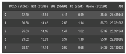
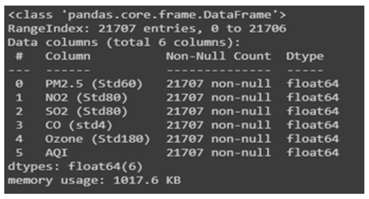
Chennai provided the data used in this analysis [20]. There are three different stations located at Manali, Velachery, and Alandur. RH, PM2.5 levels, BP, WS, and WS intensity are the wind-related variables that have been gathered from these locations for further study (WD). All stations combined produced a dataset with 35039 data rows, for a grand total of 105117 data rows, and the composed data are displayed in 15-minute intervals corresponding to the time period 2020. There was almost a 78% gap in PM2.5 data. After processing, the data was cleansed to get rid of any rows with blank columns and filtered to only include information on rows with PM 2.5 levels below 250 g/m3. Because not all rows contained the same information, we had to narrow the remaining set down to just 22827 rows. The dataset is depicted in detail in Figures 1 and 2.
Figure 1. Sample input dataset
Every 15 minutes, data on atmospheric components like, CO, and Ozone was collected from three stations spread over Chennai. Each station contributes 35039 rows of data, for a total of 490546 rows in the Dataset, covering the period of time between May 1, 2019, and April 30, 2020. Data sets are implemented to store data that may be accessed by an application. Source code, macro libraries, system variables, and parameters are all examples of data sets utilised by applications and the operating system.
Figure 2. Details of the dataset
3.2 Pre-processing
In the first step, the data are taken from the Dataset and pre-processed to get rid of extraneous information. As a result, the input data is filtered using a pre-processing procedure to remove extraneous information. The normalisation strategy is utilised for the pre-processing stage as it is more efficient at identifying outliers and filling in missing data. The primary benefit of these methods is based on the assumption that aggregating forecasts from classifiers may allow for more accurate detection of class noise in input data. As a result, the raw data is pre-processed to obtain silent data for subsequent processing, which occasionally suppresses valuable info or leads to the info loss.
3.3 Air quality forecast perfect based on LSTM
3.3.1 Time series forecast
Both meteorological elements and the mutual limitations between pollutants have an impact on the concentration of air pollutants, in addition to the concentration of pollutants in the past. Regarding time series data, LSTM shines. To better anticipate MMS messages, we developed an LSTM-based prediction model. Here is how we characterise time series forecasting:
The concentration of particulate matter in the air is signified by P=p1, p2, ..., pT, the information of meteorological factors is signified by W=w1, w2, ..., wT, and the concentration of gaseous pollutants in the air is denoted by A=a1, a2, ..., aT; hence, R=PWA. The 15 features that make up each element r i in the set R are as follows: pm2.5.
The target prediction time series is denoted by z1=(t,t + 1,t + 2,...,t + N), whereas O z1=o1, o2, ..., os and Fz1=f1, f2, ..., fs are the experiential and forecast values of s air pollutant pointers.
Predicting the concentration of the target pollutant for the next N hours requires looking at the time series before time t, which is represented by z2=t-1, t-2, ..., t-D. O pz2, O wz2, and O az2 stand for the air quality observation consequences of particle pollutants, atmospheric factors, and gaseous pollutants, respectively, over the past D hours. The same holds true for z2 [1, T] and O pz2, O wz2, O az2, R. were utilised to evaluate the results of the predictions. That example, RMSE and MAE have their limits, in that the same algorithm model can be used to solve multiple issues, and they cannot capture the benefits and drawbacks of this model for diverse problems. Because the data dimensions are unique across different practical applications, it is difficult to determine for which problem a given model is most suited for making predictions. As a result, the accuracy of the predictions is measured on a scale from 0 to 1. R2 is the regression, and is used to assess. Eq. (1) is provided to help with the RMSE computation. Below are the formulas for determining both MAE and R2:
$M A E=\frac{1}{m} \sum_{i=1}^m\left|y^i-p^i\right|$ (1)
$R^2=1-\frac{\sum_{i=1}^m\left(y^i-p^i\right)^2}{\sum_{i=1}^m\left(y^i-\hat{y}\right)^2}$ (2)
where, yi, pi, and yb stand for the expected, measured, and mean levels of air pollution. This is the number of samples used in the experiment, denoted by m. When the Mean Absolute Error and (RMSE) are both modest and the R2 value is high, the model error is small and the prediction presentation is good.
3.3.2 MMS prediction model
Through a process of layer-by-layer feature translation, deep learning is able to take the features of a sample in one space and convert them to a new feature space, which improves prediction, leverages massive data to learn features, and better represents the data's rich internal information. Gathering relevant information is the first stage. Using time-space analysis, we may extract the air quality time series data set R. The next step. Next, come the data entry and anticipated outcomes. The D-hours-earlier time series would be transformed into numerous 2-by-2 matrices. To facilitate LSTM's processing of input data, a computational architecture with multiple layers and an adequate number of neuron nodes was crafted. Through the network's learning and tuning, we determined which input and output layers would be most beneficial, and we shaped the function association from input to output to ensure that the resulting association was as accurate as possible. Decoding the LSTM output and obtaining the final prediction result required a completely linked layer, which was analogous to the model's output layer.
The first step is to obtain the raw data from each illustrative station in Chennai (S1, S23, S29, and S31); the second step is to apply the aforementioned MMS model to process the data in order to obtain a sequence at times T, T+1, ..., T+N (the attentiveness sequence of SO2); and the third step is to calculate the average value of each pollutant index (PM2.5)
3.3.3 Steps of MMS prediction model
Processing the data beforehand is the first stage. The raw dataset should undergo outlier removal and missing value stuffing before being fed into the model. This will reduce the likelihood of unwanted effects from the data dimension on the prediction outcome and speed up the rate at which the data converges. The range of the data has been standardised to (0, 1).
After that, you must change the file type. Synchronizing input and output sequences, as is done in supervised learning, from the original data sequence. A multivariate time series is used for analysis. The multivariate time series can be put to use by utilising.
Third, initialise the LSTM's parameters by splitting the data into a training and testing set. Limiting the number of generations, configuring the sum of neurons, and determining the size of the fully linked network all require setting the epoch. The process of training an LSTM model involves selecting an appropriate, loss function, and optimization method.
Fourth, anticipate using the perfect. Investigating how well the model does on a test set.
Output: Prediction model parameters such as maximum epoch, sum of neurons, learning rate, minibatch size, L2 regularisation should be saved.
Several hyperparameters in this study were determined with the aid of CHGSA. These hyperparameters included the number of LSTM layers, the sum of neurons in each LSTM layer, the number of fully connected layers, time lag D. In order to find the optimal parameter, we hold all other variables constant and examine how they affect the model's ability to make predictions.
3.4 Hyper-parameter optimization using Hunger Games Search (HGS) optimization algorithm
The Human Genome Project (HGS) is an example of a optimization technique. Used to tackle optimization problems subject to restrictions, it is easy to implement, stable, and competitive [21]. The HGS algorithm is predicated on the idea that animals would act in ways that best satisfy their hunger. The animals' social behaviours serve as inspiration, while their hunger dictates the extent of their foraging. Using the idea of "Hunger" as a driving force behind all human endeavours, this dynamic optimization method is based. The hunger is simulated in the HGS optimization algorithm through the use of weights that are meant to reflect how the hunger impacts the search stages. Animal logic is employed as the basis for the algorithm's operation. Animals engage in these behaviours, which are viewed as adaptively evolving in nature, because they do so in an effort to increase their chances of obtaining food.
3.4.1 The logic of search, games
Animals follow social norms that are shaped by their surroundings. The behaviour and appearance of animals are subject to rules. An animal's hunger will influence its decisions and actions. Animals' nervousness and the hunters' uneasiness both increase when they're hungry. When their energy reserves are low, animals will search for food. In order to make a clean transition between exploration and defence, they need to look for food in addition to moving across habitats. The ability to flee from predators and discover new food sources is bolstered by animals' social lives. Living in groups increases an animal's chances of survival. Animals who are in better health have a greater chance of survival in the wild because they are better equipped to find food. Nature provides its own version of "Hunger Games," where the stakes are high and each false move could be fatal. Animals' actions can be influenced not just by physical needs like hunger but also by psychological ones like fear of humans acting as predators. There is a direct correlation between the intensity of hunger and the intensity of the quest for food. This means the animal is making a greater effort to find food in the days leading up to his death. Species migrations and logical alternatives underpin the proposed optimization strategy.
3.4.2 Mathematical model
In this subsection, we present the fundamental exact equations underlying the HGS optimization procedure. As such, the mathematical model is constructed around behaviours that are driven by hunger.
Getting ready to dig in: Everyone is believed to get along and aid one another. Eq. (3) [21] provides the central equation of the proposed HGS optimization method, and it is this equation that embodies the individuals' cooperative communication:
$\begin{aligned} & X \overrightarrow{(t+1)} \\ & =\left\{\begin{array}{lr}\text { Game }_1: \overrightarrow{X(t)}\left(1+\operatorname{randn}(1)\right) & r_1<l \\ \text { Game }_2: \vec{W}_1 \vec{X}_b+R \rightarrow \vec{W}_2\left|\vec{X}_b-\overrightarrow{X(t)}\right|, & r_1>l, r_2>E \\ \text { Game }_3: \vec{W}_1 \vec{X}_b-R \rightarrow \overrightarrow{W_2}\left|\overrightarrow{X_b}-\overrightarrow{X(t)}\right|, & r_1>l, r_2<E\end{array}\right.\end{aligned}$ (3)
In Eq. (3), people are searching for both sites close to the optimal one and other locations far away from it. This guarantees that the search space is fully covered during the exploration process.
Hunger's part: Mathematical expressions of the population starving characteristics in the exploration field are provided, and W1 is determined using the formula (4) [21].
$\overrightarrow{W_1}(i)= \begin{cases}\text { hungry }(i) \frac{N}{\text { SHungry }} \times r_4 & r_2<l \\ 1, & r_3<l\end{cases}$ (4)
Meanwhile, $\vec{W}_2$ in Eq. (3) is calculated as shown in Eq. (5):
$\vec{W}_2(i)=2\left(1-e^{-\mid \text {hungry }(i)-\text { SHungry } \mid}\right)_{r 5}$ (5)
where, hungry is the hungry of the populace. r3, r4, and r5 are random values among 0 and 1. N is the population size. SHungry describes the synopsis of the populaces’ hungry feelings.
The hungry (i) can be signified exactly as shadows Eq. (6) [21]:
$\begin{aligned} & \operatorname{hungry}(i) \\ & =\left\{\begin{array}{lr}0, & \forall \operatorname{AllFitness}(i)==B F \\ \text { hungry }(i)+H, \forall \operatorname{AllFitness}(i)=B F\end{array}\right.\end{aligned}$ (6)
where, AllFitness(i) is the suitability of the present iteration. The optimal population has their hunger reduced to zero at each repetition. Meanwhile, the old population's hunger is multiplied by the new hunger (H). H values for each population are distinct from one another. Optimization using the HGS method is designated in pseudo-code form in Procedure 1.
|
Algorithm 1. Pseudo-code of HGS |
|
Initialize the parameters and positions while (t ≤ T) Calculate the fitness of all individuals Update BF, WF, Xb, BI Calculate the Hungry, W1, W2 for each individual Calculate E Update R and positions end for t = t + 1 end while eturn BF and Xb |
3.4.3 Chaotic hunger games search optimization algorithm (CHGS)
The initial population in meta-heuristic optimisation techniques is chosen at random between two given boundaries. The effectiveness of optimization algorithms relies heavily on the state of the agents at the outset. The quality of the starting population greatly affects the final product. In this study, we use chaotic maps to enhance the founding population. The idea of using chaotic maps to alter the seed population in metaheuristic algorithms was introduced [22, 23].
Based on the discussion [23], it has been shown that the logistic chaotic maps are the most computationally efficient of the modern chaotic maps; this is because they use a random initialization of statistics close to 0 and 1. Mathematical representations of this sympathetic of chaotic mapping are provided in Eq. (7).
$\begin{gathered}y_1=\text { rand }, \\ y_{i+1}=4 y_i\left(1-y_i\right), \forall i \in N\end{gathered}$ (7)
In this case, rand is a random vector between 0 and 1. As a result, the proposed CHGS optimization method uses the values produced from this kind of chaotic mapping to define its initial population, rather than the values provided by the HGS. The HGS simulation performance is enhanced by this replacement of the starting population.
After conducting a battery of tests, we settled on an LSTM architecture that included three hidden layers, each containing 150 neurons; additionally, we used a single fully-connected layer consisting of a single node. In addition, the tanh function is used as the (LSTM) model. Best results were obtained when training was limited to 100 iterations and the batch size was set to 512.
Using the air quality time series t, the prediction model attempts to approximation the concentration of during the next N hours. Based on the findings of several studies, even a very short delay may not be enough to ensure that the model receives adequate information for its long-term memory. However, if there is a long lag time, more noise from unrelated sources can enter the picture and distort the prediction. Because of this, we tested the model's prediction ability using the aforementioned three assessment indicators across the range of time lag D values. The results demonstrate that the hypothesis that "more time elapses, the less inaccuracy the model will have" is false. Even after adding more historical concentration data, the model's accuracy has not improved. Contrarily, as D grows larger, model training time increases with each epoch, and model performance degrades overall. To this end, we set D=9, and the resulting model required far less time and produced significantly fewer errors.
4.1 Model evaluation metrics
Prediction tests using the AQI index were used to validate the model and demonstrate its efficacy in assessing air quality. Overfitting occurs when too many training data points are used during model development, while underfitting occurs when too few are used. Consequently, the precision of the model depends critically on the method of data division that is used. Here, we normalised 8784 data points and used 95% of them for training and the remaining 5% for testing. To assess the accuracy of the model's predictions, we choose to use the (RMSE), mean absolute percentage error (MAPE), and R-squared (R2). The required formulae are shown in Eqns. (8)-(11).
$M A E=\frac{1}{n} \sum_{i=1}^n\left|\hat{y}_i-y_i\right|$ (8)
$R M S E=\sqrt{\frac{1}{n} \sum_{i=1}^n\left(\hat{y}_i-y_i\right)^2}$ (9)
$M A P E=\frac{100 \%}{n} \sum_{i=1}^n\left|\frac{\hat{y}_i-y_i}{y_i}\right|$ (10)
$R^2=1-\frac{\sum_{i=1}^n\left(\hat{y}_i-y_i\right)^2}{\sum_{i=1}^n\left(\bar{y}_i-y_i\right)^2}$ (11)
where, yi was either the actual value, the mean value, or any combination of the two; yi was the forecast value. The model fitting effect was enhanced as the MAE, RMSE, and MAPE values decreased. In addition, the perfect fitting impact was enhanced when R2 approached 1. Table 4 shows the statistical breakdown of the dataset, including the number of observations, means, standard deviations, null observations, 25%).
Table 4. A statistical synopsis of the dataset's exploratory variables
|
|
PM2.5 (Std60) |
NO2 (Std80) |
SO2 (Std80) |
CO (std4) |
Ozone (Std180) |
AQI |
|
count |
21707.000000 |
21707.000000 |
21707.000000 |
21707.000000 |
21707.00000 |
21707.000000 |
|
mean |
30.321609 |
12.088319 |
6.528234 |
0.703744 |
37.195119 |
22.412852 |
|
std |
38.133978 |
9.771051 |
5.782149 |
0.403747 |
36.083979 |
14.346564 |
|
min |
0.010000 |
0.010000 |
0.010000 |
0.000000 |
0.010000 |
2.871111 |
|
25% |
12.710005 |
5.670000 |
3.300006 |
0.450000 |
11.050000 |
15.11153 |
|
50% |
22.700000 |
10.31000 |
5.950000 |
0.660000 |
26.320000 |
20.075278 |
|
75% |
36.580000 |
16.17000 |
8.370000 |
0.8600 |
48.9600 |
26.445 |
|
max |
999.990000 |
312.93000 |
179.35000 |
10.000000 |
199.550000 |
359.8366 |
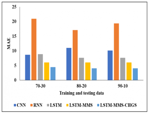
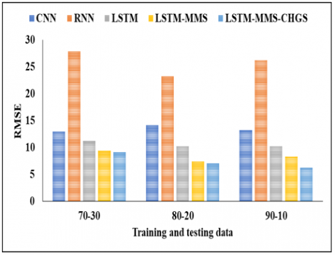
The validation analysis is based on 70%-30%, 90%-10% and 80% and 20% of training and testing data. The generic models are considered and implemented using the collected datasets and results are averaged in Tables 5 to 7.
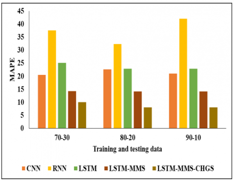
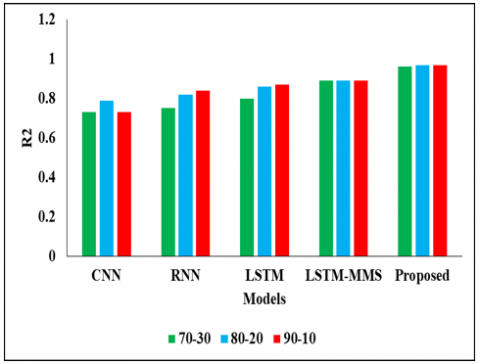
The Validation Analysis in Table 5 above is based on 70%-30% of the data. In this analysis, we have used different models such as CNN, RNN, LSTM, LSTM-MMS, and LSTM-MMS-CHGS. CNN achieved an MAE of 8.65, an RMSE of 13.02, an MAPE of 20.53 0.73, and an R2 value of 0.73 in this experimental analysis. and next the RNN reached the MAE of 20.95, the RMSE of 27.90, the MAPE of 37.62, and finally the R2 value of 0.75. The next technique, LSTM, reached the MAE value of 8.87 and also the RMSE value of 11.21, the MAPE value of 25.12, and finally the R2 value of 0.8. Another method of LSTM-MMS reached the MAE of 6.05, the RMSE of 9.43, the MAPE of 14.25, and finally the R2 value of 0.89. And finally, we evaluated the method of LSTM-MMS-CHGS and reached the MAE value of 4.42, the RMSE value of 9.12, the MAPE value of 10.05, and finally the R2 value of 0.96, respectively. By this comparison and analysis, the proposed model achieved better results than additional models.
Table 5. Validation analysis based on 70%-30% of data
|
Model |
MAE |
RMSE |
MAPE |
R2 |
|
CNN |
8.65 |
13.02 |
20.53 |
0.73 |
|
RNN |
20.95 |
27.90 |
37.62 |
0.75 |
|
LSTM |
8.87 |
11.21 |
25.12 |
0.8 |
|
LSTM-MMS |
6.05 |
9.43 |
14.25 |
0.89 |
|
LSTM-MMS-CHGS |
4.42 |
9.12 |
10.05 |
0.96 |
In the Table 6, it is represented that the analysis of various models is based on 80%-20% of the data. In this analysis, we have used different models such as CNN, RNN, LSTM-MMS, and LSTM-MMS-CHGS. In this experimental analysis, CNN reached an MAE of 11.02 and a RMSE of 14.15, as well as an MAPE of 22.64 and a final R2 value of 0.79. The RNN then achieved an MAE of 17.11, an RMSE of 23.32, an MAPE of 32.37, and an R2 value of 0.82. The next technique, LSTM, reached the MAE value of 7.62, the RMSE value of 10.21, the MAPE value of 22.87, and finally the R2 value of 0.86. Another method of LSTM-MMS reached the MAE of 6.04, the RMSE of 7.46, the MAPE of 14.13, and finally the R2 value of 0.89. And finally, we evaluate the method of LSTM-MMS-CHGS and reach the MAE value of 4.02, the RMSE value of 7.11, the MAPE value of 8.07, and finally the R2 value of 0.97, respectively. By this comparison and analysis the projected model reached the better results than other replicas.
Table 6. Analysis of various models based on 80%-20% of data
|
Model |
MAE |
RMSE |
MAPE |
R2 |
|
CNN |
11.02 |
14.15 |
22.64 |
0.79 |
|
RNN |
17.11 |
23.22 |
32.37 |
0.82 |
|
LSTM |
7.62 |
10.21 |
22.87 |
0.86 |
|
LSTM-MMS |
6.04 |
7.46 |
14.13 |
0.89 |
|
LSTM-MMS-CHGS |
4.02 |
7.11 |
8.07 |
0.97 |
Table 7 depicts the comparative analysis of the proposed model using 90%-10% of the data. In this analysis, we have used different models such as CNN, RNN, LSTM-MMS, and LSTM-MMS-CHGS. CNN achieved a MAE of 10.11, a RMSE of 13.25, a MAPE of 21.02, and an R2 value of 0.73 in this experimental analysis.The RNN then achieved a MAE of 20.95, a RMSE of 27.90, a MAPE of 37.62, and an R2 value of 0.75.The next technique, LSTM, reached the MAE value of 7.65, the RMSE value of 11.21, the MAPE value of 25.12, and finally the R2 value of 0.87. Another method of LSTM-MMS reached the MAE of 6.05, the RMSE of 9.43, the MAPE of 14.25, and finally the 21 values of 0.89. And finally, we evaluate the method of LSTM-MMS-CHGS and reach the MAE value of 4.05, the RMSE value of 6.25, the MAPE value of 8.05, and finally the R2 value of 0.97, respectively. By this comparison and analysis, the projected model achieved better results than other models. The MAE, MAPE, RMSE and R2 analysis for various training and testing data is shown in Figure 3, Figure 4, Figure 5 and Figure 6 respectively.
Table 7. Comparative analysis of proposed model using 90%-10% of data
|
Model |
MAE |
RMSE |
MAPE |
R2 |
|
CNN |
10.11 |
13.25 |
21.02 |
0.73 |
|
RNN |
19.35 |
26.25 |
42.11 |
0.84 |
|
LSTM |
7.65 |
10.25 |
22.85 |
0.87 |
|
LSTM-MMS |
6.05 |
8.32 |
14.21 |
0.89 |
|
LSTM-MMS-CHGS |
4.05 |
6.25 |
8.05 |
0.97 |
Figure 3. MAE analysis for various training and testing data
Figure 4. RMSE analysis
Figure 5. MAPE analysis for three ratios of training and testing data
Figure 6. R2 analysis
Forecasting air quality is hard because particles and gases are mobile, changeable, and hard to predict in time and place. However, the ability to analyse, forecast, and monitor air quality is becoming increasingly vital due to the critical effects of air pollution on individuals and the situation, especially in urban areas. Many cities have taken action to minimise air pollution based on AQI estimates and projections. The received dataset has been pre-processed in order to fill in any gaps and remove any extraneous data. This method makes AQI forecasts under a wide variety of weather scenarios. Then, the LSTM model is used to make an accurate prediction of the AQI in the area of interest using deep learning. With the use of the AQI, the citizens of a big city can learn about the air quality where they live. Through the application of deep learning, a precise AQI estimation was accomplished in a major city. Public transportation and road traffic signal synchronisation are two areas where the city planning committee can benefit from the expected values. In areas where pollution levels are exceptionally severe, it may be possible to switch to a system consisting solely of electrically powered or non-motorized vehicles. In metropolitan settings, these forecasts will be especially helpful in creating a sustainable community for developing nations. In the future, the AQI values of a city can be improved by using the hybrid deep learning algorithm to suggest an air pollution reduction strategy. The places most at risk from air pollution can be pinpointed using forecasted AQI values.
[1] Ravishankar, K., Devaraj, P., Hanumathaiah, S.Y. (2023). Floor segmentation approach using FCM and CNN. Acadlore Transactions on AI and Machine Learning, 2(1): 33-45. https://doi.org/10.56578/ataiml020104
[2] Liang, Y.C., Maimury, Y., Chen, A.H.L., Juarez, J.R.C. (2020). Machine learning-based prediction of air quality. Applied Sciences, 10(24): 9151. https://doi.org/10.3390/app10249151
[3] Vatambeti, R., Mantena, S.V., Kiran, K.V.D., Manohar, M., Manjunath, C. (2023). Twitter sentiment analysis on online food services based on elephant herd optimization with hybrid deep learning technique. Cluster Computing, 1-17. https://doi.org/10.1007/s10586-023-03970-7
[4] Xing, J., Zheng, S., Ding, D., Kelly, J.T., Wang, S., Li, S., Qin, T., Ma, M., Dong, Z., Jang, C., Zhu, Y. (2020). Deep learning for prediction of the air quality response to emission changes. Environmental Science & Technology, 54(14): 8589-8600. https://doi.org/10.1021/acs.est.0c02923
[5] Mao, W., Wang, W., Jiao, L., Zhao, S., Liu, A. (2021). Modeling air quality prediction using a deep learning approach: Method optimization and evaluation. Sustainable Cities and Society, 65: 102567. https://doi.org/10.1016/j.scs.2020.102567
[6] Bekkar, A., Hssina, B., Douzi, S., Douzi, K. (2021). Air-pollution prediction in smart city, deep learning approach. Journal of big Data, 8(1): 1-21. https://doi.org/10.1186/s40537-021-00548-1
[7] Kalajdjieski, J., Zdravevski, E., Corizzo, R., Lameski, P., Kalajdziski, S., Pires, I.M., Trajkovik, V. (2020). Air pollution prediction with multi-modal data and deep neural networks. Remote Sensing, 12(24): 4142. https://doi.org/10.3390/rs12244142
[8] Heydari, A., Majidi Nezhad, M., Astiaso Garcia, D., Keynia, F., De Santoli, L. (2021). Air pollution forecasting application based on deep learning model and optimization algorithm. Clean Technologies and Environmental Policy, 24: 607-621. https://doi.org/10.1007/s10098-021-02080-5
[9] Iskandaryan, D., Ramos, F., Trilles, S. (2020). Air quality prediction in smart cities using machine learning technologies based on sensor data: A review. Applied Sciences, 10(7): 2401. https://doi.org/10.3390/app10072401
[10] Chellakh, H., Moussaoui, A., Attia, A., Akhtar, Z. (2023). MRI brain tumor identification and classification using deep learning techniques. Ingénierie des Systèmes d’Information, 28(1): 13-22. https://doi.org/10.18280/isi.280102
[11] Zhang, Z., Zeng, Y., Yan, K. (2021). A hybrid deep learning technology for PM 2.5 air quality forecasting. Environmental Science and Pollution Research, 28: 39409-39422.
[12] Dairi, A., Harrou, F., Khadraoui, S., Sun, Y. (2021). Integrated multiple directed attention-based deep learning for improved air pollution forecasting. IEEE Transactions on Instrumentation and Measurement, 70: 1-15. https://doi.org/10.1109/TIM.2021.3091511
[13] Zhao, Z., Wu, J., Cai, F., Zhang, S., Wang, Y.G. (2022). A statistical learning framework for spatial-temporal feature selection and application to air quality index forecasting. Ecological Indicators, 144: 109416. https://doi.org/10.1016/j.ecolind.2022.109416
[14] Middya, A.I., Roy, S. (2022). Pollutant specific optimal deep learning and statistical model building for air quality forecasting. Environmental Pollution, 301: 118972. https://doi.org/10.1016/j.envpol.2022.118972
[15] Haq, M.A. (2022). Smotednn: A novel model for air pollution forecasting and aqi classification. Computers, Materials & Continua, 71(1): 1403-1425. https://doi.org/10.32604/cmc.2022.021968
[16] Zeng, Y., Chen, J., Jin, N., Jin, X., Du, Y. (2022). Air quality forecasting with hybrid LSTM and extended stationary wavelet transform. Building and Environment, 213: 108822. https://doi.org/10.21203/rs.3.rs-357905/v1
[17] Wu, C.L., Song, R.F., Zhu, X.H., Peng, Z.R., Fu, Q.Y., Pan, J. (2023). A hybrid deep learning model for regional O3 and NO2 concentrations prediction based on spatiotemporal dependencies in air quality monitoring network. Environmental Pollution, 121075. https://doi.org/10.1016/j.envpol.2023.121075
[18] Ding, L., Sun, J., Shen, T., Jing, C. (2023). A noval air quality index prediction scheme based on long short-term memory technology. In Advances in Natural Computation, Fuzzy Systems and Knowledge Discovery: Proceedings of the ICNC-FSKD 2022, pp. 43-52. https://doi.org/10.1007/978-3-031-20738-9_6
[19] Aarthi, C., Ramya, V.J., Falkowski-Gilski, P., Divakarachari, P.B. (2023). Balanced spider monkey optimization with Bi-LSTM for sustainable air quality prediction. Sustainability, 15(2): 1637. https://doi.org/10.3390/su15021637
[20] Janarthanan, R., Partheeban, P., Somasundaram, K., Elamparithi, P.N. (2021). A deep learning approach for prediction of air quality index in a metropolitan city. Sustainable Cities and Society, 67: 102720. https://doi.org/10.1016/j.scs.2021.102720
[21] Yang, Y., Chen, H., Heidari, A.A., Gandomi, A.H. (2021). Hunger games search: Visions, conception, implementation, deep analysis, perspectives, and towards performance shifts. Expert Systems with Applications, 177: 114864. https://doi.org/10.1016/j.eswa.2021.114864
[22] Shaheen, M.A.M., Hasanien, H.M., El Moursi, M.S., El-Fergany, A.A. (2021). Precise modeling of PEM fuel cell using improved chaotic MayFly optimization algorithm. International Journal of Energy Research. https://doi.org/10.1002/er.6987
[23] Gao, J., Ismail, N., Gao, Y.J. (2022). Computer big data analysis and predictive maintenance based on deep learning. Ingénierie des Systèmes d’Information, 27(2): 349-355. https://doi.org/10.18280/isi.270220