Fatima Moulay* | Assia Habbati | Abdelkader Lousdad
© 2022 IIETA. This article is published by IIETA and is licensed under the CC BY 4.0 license (http://creativecommons.org/licenses/by/4.0/).
OPEN ACCESS
The objective of this paper is to present the modelling and simulation of the PV generation system connected to the network under MATLAB/Simulink. Firstly, a mathematical model of the Photovoltaic Module is developed taking meteorological data namely the irradiance and temperature as input variables needed to model this device. The output can be current, voltage or power. The model allows the prediction of the behavior and characteristics of the PV module based on the equivalent circuit of the mathematical model under different temperatures and solar radiation readings. Secondly the PV array is connected to the boost DC-DC converter, the control systems based on Maximum Power Point Tracking (MPPT) with P&O algorithm helps the PV array to generate the maximum power to the grid in case of changing weather conditions, then in the third step, it is integrated into AC power grid by DC/AC inverter to control active and reactive power to achieve unity power factor which is validated by satisfactory results. In this paper, different cases are simulated and the results verified the validity of the models.
irradiance, PV modelling, boost converter, perturb and observe, PV array, grid, MPPT control, power inverter
Today, photovoltaic technology is sufficiently mature and mastered to really take off in the field of energy power applications, as well as the optimization of systems. Photovoltaic surely leads to a better exploitation of solar energy [1].
The photovoltaic generator is the only direct converter to transform solar radiation into electrical energy.
However, the photovoltaic generator is not able to generate energy suitable for the load nor the connection to the electricity grid. Always use one or two adaptation stages [2].
It is the role of power converters that are as important as they are indispensable in photovoltaic systems.
There are several types of converters:
Generally, two converters are necessary to adapt the energy produced by the photovoltaic generator; a DC / DC converter to raise or lower the voltage to the desired value and an inverter to switch from the continuous form delivered by the photovoltaic generator to the alternating form [3].
Research has been done to improve power converters from a techno-economic point of view leading to a new created alternative. It is the combination of two DC / DC boost converters and inverter [4].
Later, in the 2000s, a new technology appeared with the DC/AC converter of impeding-source inverter types. The aim was to improve the energy efficiency of the photovoltaic generator.
In this regard, the work carried out in this paper is devoted to the modeling and simulation of a photovoltaic conversion chain composed of a PV field, a boost converter, an inverter, a load and a three-phase network [5].
The choice of this configuration is intended to boosting the direct voltage obtained from the photovoltaic generator as well as making it compatible with that of the network.
The role of the first part of the designed system consists in extracting the maximum power from the photovoltaic field by means of the MPPT technique [6].
The converter used is either a voltage boost or boost converter. Its control is done by a script that varies the duty cycle by a three-phase voltage inverter [7].
Several regulation systems are required to control and regulate the amplitude of the DC bus voltage at the input of the inverter as well as the amplitude and frequency of the AC voltage at its output [8].
An adaptation stage with an MPPT function has also been inserted between the photovoltaic generator and the inverter in order to constantly optimize the produced power.
Based on the literature studies of various references related to the subject had reveal that the multiplication of the adaptation stages allows a maximization of the available power but to the detriment of the global conversion efficiency. Therefore, the compromise between a maximum of power and a decrease in global efficiency is a technological challenge that resides in the search for solutions related to photovoltaic energy, this consists in considering the right management architectures much more for the DC-DC adaptation stages (Converters) than for DC-AC (inverters) [9].
The most favourable topology is the very low power adaptation stage (micro-converters) which operates as close as possible to the photovoltaic module.
A two-stage adaptation simulation has been developed in this investigation. The first is a boost type voltage lifting structure. The second is an inverter that delivers a sinusoidal voltage suitable for both loads and connection to the power grid.
In this work the photovoltaic conversion chain connected or not to the network, and, either with or without storage (batteries) is considered.
In the first part, the description and the modeling of the PV module is given. The second part exposes the principle of operation and the analysis of the MPPT method. In the third part the structural development is made and the description is given for the interactive PV system to the proposed network which includes PV panels, a VSI, a filter, a transformer and a controller dealing with the implementation of active and reactive power flow control.
The analysis and discussion of the obtained results of the simulation as well as the conclusion are given in the final part.
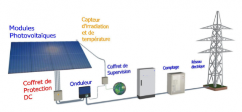
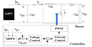
The systems connected to the grid is shown in (Figure 1) or "grid-connected". The parallel connection of the system to the public electricity grid is intended to inject into the grid, the electrical energy produced by the photovoltaic fields. In Grid-Connected Systems, standard power consumers are connected to the generator via an inverter (DC-AC converter) The task of the inverter is to transform the direct current coming out of the panels into an alternating current. In grid-connected systems, the inverter replaces the batteries, in this case, it is the basic element in these types of systems [10].
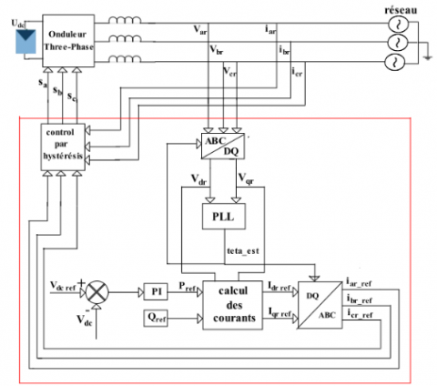
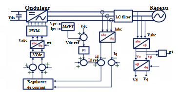
Figure 2 presents a general diagram showing where the components of the current are, compared with the references. The intervals between them go through the regulators [7]. The outputs of the regulators give the components of the reference voltage of the PWM in the mark d-q. Going through the inverse transformation of Park, we obtain the references of the PWM control signal of the switches of the inverter [8].
For the moment, in most of the countries where the connection is authorized and regulated, the current cost of photovoltaic technology is much higher than that of traditional energy [11]. It is difficult to say how long it will take to reach a price level where photovoltaic kWh will be competitive with conventional kWh, derived from fossil fuels (oil, gas or coal) or fissile (nuclear).
Figure 1. Diagram of a grid-connected photovoltaic system
Figure 2. Synoptic diagram of the connection of the inverter to the electrical network
The PV modules are assembled in long series called chains which designate the word "strings" in English. At the beginning of the connection of PV installations to the grid, this topology was widely used because it made it possible to deliver a voltage to the DC bus high enough without amplifying it by a DC / DC device such as the chopper. This central inverter offers high energy efficiency at low costs. Everything is connected to the grid via a single inverter. At high power greater than 10KW (> 10KW) the efficiency of the inverter is unbeatable (95% to 97%). But this yield can only be achieved under optimal conditions. It is reduced when all the modules do not have the same characteristics. A cloud that overshadows a few modules, or for some reason some modules are dirty or have aged or compared to others. The other disadvantage of this centralized inverter is the losses caused by the high voltage DC cable which connects all the PV modules to the inverter [12].
These losses are significant because the MPPT located in the inverter forces the PV generator to operate at maximum power. In addition, the use of a single inverter for all PV modules remains a disadvantage. Similar to putting all your eggs in one basket [13].
In central inverters, usually, a large inverter is used to convert power on the (DC-DC) side of the (PV) modules to power (AC) on the AC side. In this system, the modules of (PV) are in series to form a panel, and several of these panels are connected in parallel to the chopper [14].
4.1 PV generator model
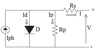
There are different types of solar (photovoltaic) cells, and each type of cell has its own performance and cost [15]. In this paper, we study the one-diode model where the cell is presented as an electric current generator whose behaviour is equivalent to a current source given by the Figure 3.
Figure 3. Electrical model of the cell
In this case, the Kirchhoff nodes law Figure 3:
$I=I_{p \hbar}-I_{d}-I_{p}$ (1)
The leakage current $I_{p}$ is deduced from the diagram by applying the law of the meshes of Kirchhoff:
$I_{p}=\frac{V+R_{s} I}{R_{p}}$ (2)
The photocurrent is given by:
$I_{p h}=\left(\frac{G}{G_{r e f}}\right)\left(I_{p h, r e f}+\mu c c\left(T_{c}-T_{c, r e f}\right)\right)$ (3)
The diode current is given by:
$I_{d}=I_{0}\left[\exp \left(\frac{e\left(V+I R_{s}\right.}{\lambda K T_{c}}\right)-1\right]$ (4)
The inverse saturation current is defined by the following formula [6]:
$I_{0}=D T_{c}^{3} \exp \left(\frac{-e \varepsilon_{G}}{n K T_{c}}\right)$ (5)
In order to eliminate the term D, the saturation current is calculated twice; at $T_{c}$ and $T_{c, r e f}$, then the two equations are divided into parts:
$I_{0}=I_{0, \text { ref }}\left(\frac{T_{c}}{T_{c, \text { ref }}}\right)^{3} \exp \left[\left(\frac{e \varepsilon_{G}}{n K}\right)\left(\frac{1}{T_{c, \text { ref }}}-\frac{1}{T_{c}}\right)\right]$ (6)
It is necessary to write the characteristic equation I (V):
$I=I_{p h}-I_{0}\left[\exp \left(\frac{e\left(V+R_{s} I\right.}{\lambda K T_{c}}\right)-1\right]-\frac{V+R_{s} I}{R_{p}}$ (7)
We can write the following three relations:
$I_{c c, \text { ref }}=I_{p h, r e f}-I_{0, \text { ref }}\left[\exp \left(\frac{e I_{c c, r e f} \,\,\,\,R_{s}}{\lambda K T_{c, r e f}}\,\,\,\right)-1\right]$ (8)
$0=I_{p h, r e f}-I_{0, \text { ref }}\left[\exp \left(\frac{e V_{c o, r e f}}{\lambda K T_{c, e f}}\right)-1\right]$ (9)
$I_{p m, r e f}=I_{p h, r e f}-I_{0, r e f}\left[\exp \left(\frac{e\left(V_{p m, r e f}\,\,\,\,+I_{p m, r e f} \,\,\,\,R_{s}\right.}{\lambda K T_{c, \text { ref }}}\,\,\,\right)-1\right]$ (10)
Since the saturation, current is of the order of $10^{-6}$ and less, it minimizes the impact of the exponential in Eq. (8), so it can be deduced that:
$I_{c c, r e f} \approx I_{p h, r e f}$ (11)
By replacing $I_{p h, r e f}$ with $I_{c c, \text { ref }}$ in Eq. (9):
$0 \approx I_{c c, r e f}-I_{0, \text { ref }} \exp \left(\frac{e V_{c o, r e f}}{\lambda K T_{c, r e f}}\right)$ (12)
$I_{0, r e f}=I_{c c, r e f} \exp \left(\frac{-e V_{c o, r e f}}{\lambda K T_{c, r e f}}\right)$ (13)
For the calculation of $I_{0}$, we replace in Eq. (6) and for $I_{p h}$ in Eq. (3).
4.2 Simulations results
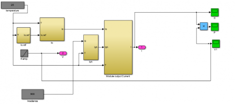
To simulate our photovoltaic generator, we plug in Simulink/ Matlab, the blocks which characterize the equations of the model and we simultaneously vary the irradiance and the temperature in the following Figure 4.
Figure 4. PV module in MATLAB/Simulink
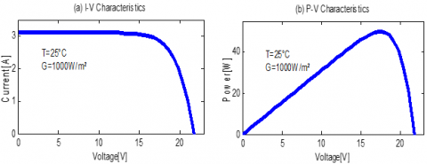
The characteristic I (V) represented by Eq. (7) made it possible to draw the curves of the variation in I–V and P–V characteristics which are shown in Figure 5.
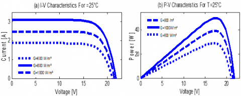
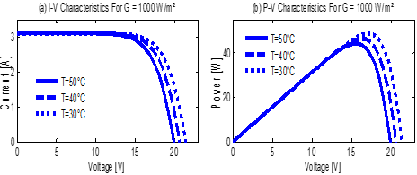
Figures 6 and 7 represent respectively the current-voltage and power-voltage characteristics.
Figure 5. (a) I–V and (b) P–V characteristics for G and T Constants
Figure 6. (a) I–V and (b) P–V characteristics for T constant
Figure 7. (a) I–V and (b) P–V characteristics for G constant
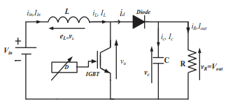
Boost topology is used to increase voltage, it is given by Figure 8.
Figure 8. Electrical circuit of a Boost chopper
The best-known topologies in the majority of applications are Fly-back, half-bridge and full-bridge [16].
Table 1 summarizes the main transformation ratios according to the duty cycle for the different structures of static converters with and without galvanic isolation. Where D is the converter duty cycle and K is the isolation transformer transformation ratio [17].
Table 1. Transformation ratios according to the duty cycle
|
Converter |
Transformation ratio according to (D) |
Galvanic isolation |
|
Buck |
D |
No |
|
Boost |
$\frac{1}{1-D}$ |
No |
|
Buck Boosts |
$\frac{-D}{1-D}$ |
No |
|
Fly backs |
$K \frac{D}{1-D}$ |
Yes |
The high cost of the photovoltaic generator imposes an optimal use and rationality of the latter to achieve an economical and profitable operation. For this, we have to use the PV generator in the region where it delivers its maximum power [18].
There are many methods to control the power delivered by the photovoltaic generator but they all remain dependent on the measurements of the parameters of the generator. There are two main categories; direct control and indirect control.
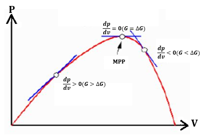
The principle of P&O type MPPT controls (Figure 9), consists in perturbing the voltage Vpv or the current Ipv with a small value and analysing the behaviour of the resulting power variation Ppv. However, these methods present some problems linked to the oscillations around the PPM.
Figure 9. The power characteristic of the PV generator
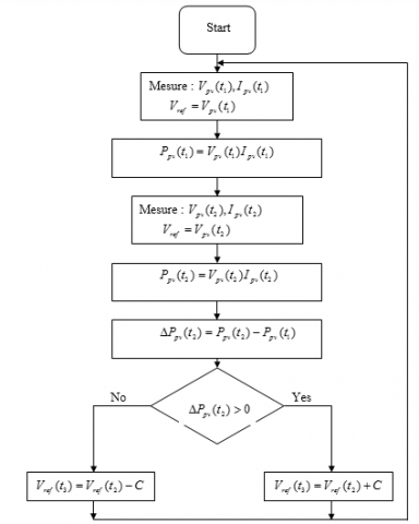
The algorithm of the P&O method is presented in the following Figure 10 [10].
It only requires measurements on the panel's output voltage Vpv and its output current Ipv. It can immediately detect the maximum power point by generating a voltage Vref at its output.
Figure 10. The algorithm of the P&O method
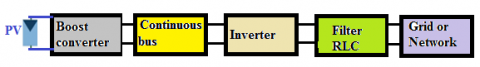
The simulation aims to determine the role of the inverter of the photovoltaic chain connected to the low voltage electricity grid [19]. The system contains a PV array, followed by two adaptation stages: a boost converter and a three-phase inverter. The simulation is carried out under MATLAB-Simulink.
Figure 11 presents the synoptic diagram of the studied system.
Figure 11. Synoptic diagram of the system
The system is composed of:
The photovoltaic generator must produce a direct voltage of nearly 300V. This voltage is boosted to 600V at the input of the inverter. Frequency at the output of the inverter is regulated using the control and regulation loops at the frequency of the network, which is 50Hz. The system must deliver a voltage.
7.1 Photovoltaic field
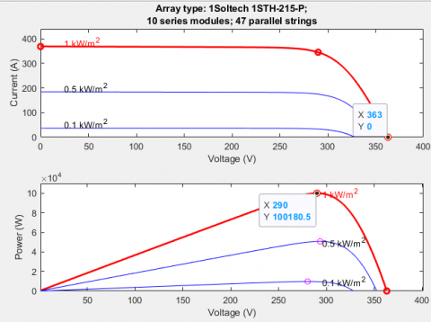
A version was used which has in its library the model of the Simulink block PV array ready, which gives a large choice among the PV modules on the market. You can change the temperature just as you can change the irradiance. For each choice, a graph shows the shape of the characteristics I (V) and P (V) by indicating the coordinates of the maximum power point (Figure 12).
We chose to connect to the grid a photovoltaic field generating maximum power of 100 kW in climatic conditions of 1000w / m2 of irradiance and 25℃.
The PV field is made up of 47 branches in parallel, each made up of 10 modules in series.
The voltage corresponding to the maximum power is 290 V.
Figure 12. Characteristic of the photovoltaic field installed in Matlab
The characteristics of the chosen module are summarized in Table 2.
Table 2. Photovoltaic module characteristic
|
Symbol |
Size (Unit) |
|
VCO |
36.3 (V) |
|
ICC |
7.84 (A) |
|
VMPP |
29 (V) |
|
IMPP |
7.35 (A) |
|
PM |
231.15 (W) |
|
Ncell |
60 (Ncell) |
7.2 Converter
The control of the booster converter is based essentially on the optimum value of the power generated by the PV field. Voltage and current corresponding to this power will be used by the algorithm presented by its script a little further, they will help extract the best value to optimize the efficiency of the PV generators [20]. The following Figure 13 shows a basic diagram of the converter control [21].
Figure 13. Boost circuit and its control
7.3 Inverter
In the chain of the PV generator connected to the grid, the inverter is placed downstream from the converter. The following Figure 14 is a diagram showing the main voltage and current control loops [22]. There is a very important condition to be fulfilled: synchronize the output of the inverter with the network and impose the frequency of the network at its output so that it does not adopt that of the load, which is often very polluting [23].
Figure 14. Control of a three-phase inverter connected to the grid
7.4 Active and reactive power flow control
The three essential inputs to the control subsystem are the voltage and current delivered by the network as well as the voltage delivered by the photovoltaic field [24, 25].
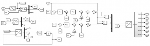
The working principle of the control is to obtain the voltages Vd, Vq and the currents Id, Iq, obtained by transformation of Park and Clarke to obtain a reference voltage used to control the inverter (Figure 15).
The control strategy mainly consisted of the DC/AC converter is designed to supply current into the utility line by regulating the bus voltage.
Figure 15. Control subsystem
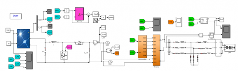
Figure 16. Main diagram of the system produced using Matlab-Simulink
In the power DC-AC converters active and reactive power from the grid-side inverter can be given by:
$P=\frac{3}{2}\left(\mathrm{v}_{\mathrm{d}} \mathrm{i}_{\mathrm{d}}+\mathrm{v}_{\mathrm{q}} \mathrm{i}_{\mathrm{q}}\right)$ (14)
$P=\frac{3}{2}\left(\mathrm{v}_{\mathrm{q}} \mathrm{i}_{\mathrm{d}}-\mathrm{v}_{\mathrm{d}} \mathrm{i}_{\mathrm{q}}\right)$ (15)
The following Figure 16 shows the main assembly made with Matlab-Simulink. It comprises a photovoltaic field with two inputs here considered fixed. They represent irradiance and temperature. It is the meteorological data that goes into the modelling of the photovoltaic module which is not represented in this work.
The electrical network block is preceded by a three-phase measuring device which collects the three-phase voltage and current to use them as references in the regulation of the inverter.
The diagram also shows a load and filters as well as subsystems.
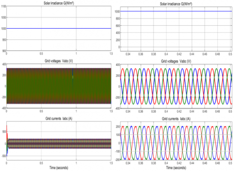
Figure 17 shows the three-phase voltage and current on the network side. Zoom is performed for the sake to highlight the sinusoidal aspect of the two shapes.
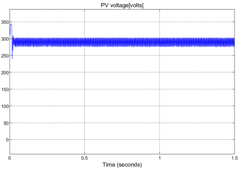
Figure 18 shows the shape of the voltage at the output of the photovoltaic generator. Note that as the irradiance has not been modified, the voltage obtained corresponds to that indicated on the graph of the characteristics of the photovoltaic field installed in Matlab which is 290V.
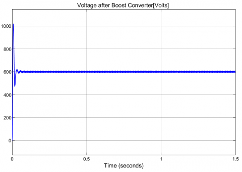
The output voltage of the converter is shown in Figure 19.
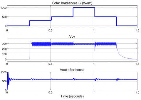
Figure 20 shows the characteristics of the photovoltaic field installed in Matlab and which is 290V and the output voltage by varying irradiances.
Figure 17. The output voltage of the PV generator
Figure 18. Three-phase network voltages and currents
Figure 19. Converter output voltage
Figure 20. Output voltage of the photovoltaic generator and Boost Converter by varying irradiance
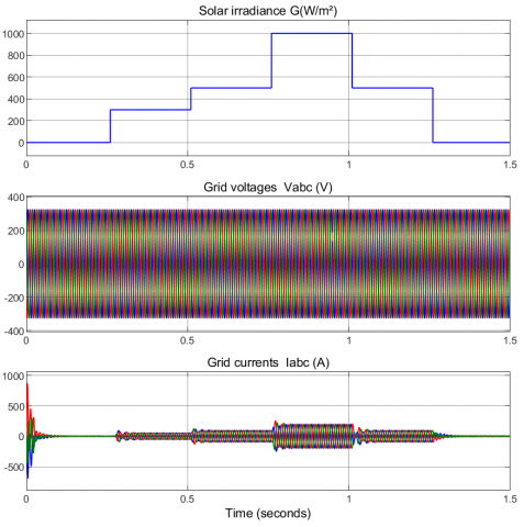
Figure 21. Three-phase network voltages and currents by varying the irradiance
The voltage value is 290 V at t = 0.25 s.
We have the same reference 600 volts of the voltage after boost. The fluctuations appear when we change the irradiation.
The current change with the expecting irradiation is shown in Figure 21.
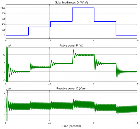
Figure 22. PV output power P and reactive power Q by varying irradiance
The DC-link voltage is compensated by the MPPT scheme for any variation in solar irradiation to maximize the output power.
The input power P rapidly and accurately reaches the maximum power corresponding to Vmpp. This can reveal and demonstrate the importance of the MPPT algorithm performance in the resolution of the problem of the degradation of the climatic factors as shown in Figure 22.
In this paper, an approach of modelling and simulation under Matlab/Simulink of a solar or photovoltaic system is presented. The system makes it possible to supply a load as it can be connected to the low voltage alternating electrical network.
This work presents a technique for the design and control of a grid-connected PV generation system by identifying its components and describing its operation. In order to convert solar energy efficiently, the MPPT algorithm for photovoltaic systems based on the P&O algorithm was presented and implemented. The approach should be followed to ensure that the photovoltaic generator generates the most energy to the electrical grid and describes the following control algorithms used for the DC-AC inverter to regulate active and reactive power to achieve the power factor unitary. All the simulation results obtained under the Matlab/Simulink environment show that the control performance and the dynamic behavior of the grid-connected photovoltaic system provide good results and show that the control system is robust, efficient and reliable.
|
I |
Current delivered by the module |
|
$I_{p h}$ |
Photocurrent |
|
$I_{d}$ |
Diode (saturation) current |
|
$I_{p}$ |
Leakage current in the shunt resistor (parallel) |
|
$R_{p}$ |
Shunt resistance (parallel) |
|
G |
Irradiance |
|
$G_{r e f}$ |
Irradiance in standard conditions = 1000W / m2 |
|
$T_{c, r e f}$ |
Temperature of the cell under standard conditions = 25℃ |
|
$\mu c c$ |
Coefficient of temperature of the DC current given by the manufacturer (A / ℃) |
|
$I_{p h, r e f}$ |
Photocurrent in the standard conditions |
|
V |
Voltage at the terminals of the module |
|
$R_{s}$ |
Contact resistance of the grids with the surfaces of the cells and the resistance of the material (series resistance) |
|
$I_{0}$ |
Saturation current |
|
K |
Boltzmann constant |
|
D |
Diffusion factor of the diode |
|
Greek symbols |
|
|
$\lambda$ |
Product of the number of cells in series of the module (A) by the quality factor (n) |
|
e |
Charge of the electron |
|
$\mathcal{\varepsilon}_{G}$ |
Width of the forbidden band (eV) |
[1] Al-Shetwi, Q., Sujod, M.Z., Ramli, N.L. (2015). A review of the fault ride through requirements in different grid codes concerning penetration of PV System to the electric power network. ARPN Journal of Engineering and Applied Sciences, 10(21): 9906-9912.
[2] Subudhi, M.B., Pradhan, R. (2013). A comparative study on maximum power point tracking techniques for photovoltaic power systems. Sustainable energy. IEEE Transactions on Sustainable Energy, 4(1): 89-98. https://doi.org/10.1109/TSTE.2012.2202294
[3] Huynh, D.C., Nguyen, T.N., Dunnigan, M.W., Mueller, M.A. (2013). Dynamic particle swarm optimization algorithm based on maximum power point tracking of solar photovoltaic panels. In Industrial Electronics (ISIE), 2013 IEEE International Symposium. pp. 1-6. https://doi.org/10.1109/ISIE.2013.6563616
[4] Kumari, J.S., Babu, D.C.S., Babu, A.K. (2012). Design and analysis of P&O and IP&O MPPT technique for photovoltaic system. International Journal of Modern Engineering Research, 2(4): 2174-2180.
[5] Kollimalla, S.K., Mishra, M.K. (2014). Variable perturbation size adaptive P&O MPPT algorithm for sudden changes in irradiance. Sustainable Energy, IEEE Transactions, 5(3): 718-728. https://doi.org/10.1109/TSTE.2014.2300162
[6] Bellia, H., Youcef, R., Fatima, M. (2014). A detailed modeling of photovoltaic module using MATLAB NRIAG. Journal of Astronomy and Geophysics, 3(1): 53-61. https://doi.org/10.1016/j.nrjag.2014.04.001
[7] Makhlouf, M., Messai, F., Benalla, H. (2012). Modeling and control of a single-phase grid-connected photovoltaic system. Journal of Theoretical and Applied Information Technology, 37(2): 289-296.
[8] Dris, M., Djilani, B. (2018). Hybrid system power generation wind-photovoltaic connected to the electrical network 220 kV. International Journal of Applied Power Engineering (IJAPE), 7(1): 10-17. http://doi.org/10.11591/ijape.v7.i1.pp10-17
[9] Kumar, A., Sadhu, P.K., Singh, J. (2021). Implementation and comparative analysis of time equivalent space vector PWM method for 3 phase to 3 phase matrix converter. Journal Européen des Systèmes Automatisés, 54(4): 617-622. https://doi.org/10.18280/jesa.540411
[10] El Halim, A.A.E.B., Bayoumi, B. (2021). Using a new combination of P&O and ICM methods for the experimental validation of MPPT efficacy. Journal Européen des Systèmes Automatisés, 54(6): 797-804. https://doi.org/10.18280/jesa.540601
[11] Lorenzini, G., Kamarposhti, M.A., Solyman, A.A.A. (2021). Maximum power point tracking in the photovoltaic module using incremental conductance algorithm with variable step length. Journal Européen des Systèmes Automatisés, 54(3): 395-402. https://doi.org/10.18280/jesa.540302
[12] Adhya, S., Saha, D., Das, A., Jana, J., Saha, H. (2016). An IoT based smart solar photovoltaic remote monitoring and control unit. 2nd International Conference on Control, Instrumentation, Energy & Communication (CIEC). https://doi.org/10.1109/ciec.2016.7513793
[13] Moreno-Garcia, I.M., Palacios-Garcia, E.J., PallaresLopez, V., Santiago, I., Gonzalez-Redondo, M.J., VaroMartinez, M., Real-Calvo, R.J. (2016). Real-time monitoring system for a utility-scale photovoltaic power plant. Sensors, 16(6): 770. https://doi.org/10.3390/s16060770
[14] Ortega, E., Aranguren, G., Saenz, M.J., Gutierrez, R., Jimeno, J.C. (2017). Study of photovoltaic systems monitoring methods. 2017 IEEE 44th Photovoltaic Specialist Conference (PVSC). https://doi.org/10.1109/pvsc.2017.8366523
[15] Van Sark, W., Louwen, A., Tsafarakis, O., Moraitis, P. (2017). PV System monitoring and characterization. Photovoltaic Solar Energy, 553-563. https://doi.org/10.1002/9781118927496.ch49
[16] Tiandho, Y., Sunanda, W., Afriani, F., Indriawati, A., Handayani, T.P. (2018). Accurate model for temperature dependence of solar cell performance according to phonon energy correction. Latvian Journal of Physics and Technical Sciences, 55(5): 15-25. https://doi.org/10.2478/lpts-2018-0032
[17] Dubey, S., Sarvaiya, J.N., Seshadri, B. (2013). Temperature dependent photovoltaic (PV) efficiency and its effect on PV production in the world–A review. Energy Procedia, 33: 311-321. https://doi.org/10.1016/j.egypro.2013.05.072.
[18] Park, N.C., Oh, W.W., Kim, D.H. (2013). Effect of temperature and humidity on the degradation rate of multicrystalline silicon photovoltaic module. International Journal of Photoenergy, 1-9. https://doi.org/10.1155/2013/925280
[19] Tijjani Baraya, J., Hamza Abdullahi, B., Sylvester Igwenagu, U. (2020). The effect of humidity and temperature on the efficiency of solar power panel output in Dutsin-ma local government area (L.G.A), Nigeria. Journal of Asian Scientific Research, 10(1): 1-16. https://doi.org/10.18488/journal.2.2020.101.1.16
[20] Sunanda, W., Tiandho, Y., Gusa, F.R., Darussalam, M., Novitasari, D. (2021). Monitoring of photovoltaic performance as an alternative energy source in campus buildings. Instrumentation Mesure Métrologie, 20(3): 153-159. https://doi.org/10.18280/i2m.200305
[21] Hamied, A., Mellit, A., Zoulid, M.A., Birouk, R. (2018). IoT-based experimental prototype for monitoring of photovoltaic arrays. In 2018 International Conference on Applied. https://doi.org/10.1109/icass.2018.8652014
[22] Loukriz, A., Saigaa, D., Drif, M., Hadjab, M., Houari, A., Messalti, S., Saeed, M.A. (2021). A new simplified algorithm for real-time power optimization of TCT interconnected PV array under any mismatch conditions. Journal Européen des Systèmes Automatisés, 54(6): 805-817. https://doi.org/10.18280/jesa.540602
[23] Van Sark, W., Louwen, A., Tsafarakis, O., Moraitis, P. (2017). PV System monitoring and characterization. Photovoltaic Solar Energy, 553-563. https://doi.org/10.1002/9781118927496.ch49
[24] Rani, B.I., Ilango, G.S., Nagamani, C. (2013). Enhanced power generation from PV array under partial shading conditions by shade dispersion using Su Do Ku configuration. IEEE Transactions on Sustainable Energy, 4(3): 594-601. https://doi.org/10.1109/TSTE.2012.2230033
[25] Deshkar, S.N., Dhale, S.B., Mukherjee, J.S., Babu, T.S., Rajasekar, N. (2015). Solar PV array reconfiguration under partial shading conditions for maximum power extraction using genetic algorithm. Renewable and Sustainable Energy Reviews, 43: 102-110. https://doi.org/10.1016/j.rser.2014.10.098