Muh. Galib Ishak | I Gede Tunas* | Rudi Herman | Setiyawan | Yassir Arafat
© 2021 IIETA. This article is published by IIETA and is licensed under the CC BY 4.0 license (http://creativecommons.org/licenses/by/4.0/).
OPEN ACCESS
2D hydrodynamic simulation is very important to be performed to interpret the flow characteristics of a river segment. The success of this simulation is determined not only by the input boundary data, but also by the quality of the data used to create the geometry model, such as terrestrial survey data, digital elevation model (DEM) or data from other sources. This paper aims to assess the use of National DEM data (DEMNAS) as the basis for constructing a 2D geometry model for flow simulation in the downstream segment of the Palu River, Sulawesi, Indonesia. The simulation results using this DEM were compared with simulations based on geometry generated from terrestrial survey data. The hourly observation discharge data at Point P3 and tidal observation data at Point P1 in the period March 17th – 18th, 2021 were assigned as the inputs at the upstream and downstream boundaries, respectively. The performance of the two model scenarios was evaluated by comparing the water surface elevation observed and simulated during the time range at Point P2 using the efficiency of Nash–Sutcliffe (NSE). The simulation results show that the two geometry-forming data provide different performance against NSE. The terrestrial survey data shows a fairly good performance, while the DEMNAS data indicates a poor performance with a negative NSE. Based on the NSE of these two scenarios, it can be interpreted that the DEMNAS data is still not sufficient to construct the model geometry for the case in this area. This is not only related to the DEMNAS resolution, especially the vertical resolution, but is also related to the very low topographical slope in the estuary of the river. However, the use of these data in areas of higher slope can be re-evaluated.
hydrodynamic simulation, RMA2, mesh, bed geometry, DEMNAS data
In line with the development of computer technology at this time, mathematical modeling to analyze the behavior of a parameter or variable in natural phenomena is a priority of choice, including the field of hydrodynamics for flow analysis in rivers [1]. Flow simulations in rivers are generally performed in connection with the changes in flow characteristics such as velocity, flow depth and sediment transport. These parameters play an important role in controlling channel changes and riverbed morphology [2]. Changes in the characteristics of these parameters are very important to be predicted continuously through hydrodynamic simulations, especially based on two-dimensional (2D) approach. This Information can be used as a reference in river management to reduce the negative impacts it causes. Pollution, siltation, erosion of cliffs or grooves and flooding are some of the bad impacts due to river exploitation in the upstream, middle and estuary segments [3].
This model provides satisfactory results on high resolution topographic data known as DEM [4-7]. DEM is a spatial elevation data that represents a 3D topographic surface which consists of coordinates and elevation in the form of grids, triangulated irregular networks (TIN) and contours. High resolution DEM is very rarely available for updates and can only be accessed at a relatively expensive cost. DEMs published for free by various spatial information agencies in the world are generally medium to low resolution and are not updated. However, apart from being freely accessible, this DEMs coverage covers almost the entire world, including Indonesia. A number of countries have provided high-resolution DEMs for their area. Indonesia through The Indonesian Geospatial Information Agency has also published DEMNAS for areas in Indonesia, which is established from a combination of several types of medium DEM such as TERRASAR-X (5m resolution), IFSAR (5m resolution) and ALOS PALSAR (11.25m 5m resolution) [8].
The use of DEM data as a basis for forming geometry for flow modeling has been carried out by many researchers, both for hydrological and hydrodynamic modeling. The application of this data for hydrological modeling, especially the rainfall-runoff transformation at the watershed scale, generally shows good performance as done by Tunas (2019) [9]. The use of similar data with various resolutions also indicates quite satisfactory results for hydrodynamic simulations in rivers. Researchers such as Mandlburger et al. (2009) [10], Shen et al. (2015) [11], Tunas and Maadji (2018) [12], and Li et al. (2020) [13] have performed a flow simulation on a river using geometry from LIDAR data and various other DEM data. Almost all of these simulations show good performance with respect to the DEM data used with a resolution of less than 5 meters. In addition, most of the simulations are assigned to areas with moderate to high slope topography.
This paper aims to evaluate the application of DEMNAS as the basis of model geometry at the mouth of the Palu River, Sulawesi, Indonesia. Based on a number of publications, the DEM data with a spatial resolution of 0.27-arcsecond has never been evaluated for hydrodynamic modeling in rivers. Previous publications only mentioned this DEM examination for watershed modeling with high performance. The results of this study will be important as a reference in using DEM data for similar studies. Information from this paper can also trigger the provision of DEM data with better resolution with free access rights, primarily to support hydrodynamic simulations.
2.1 Description of the research site
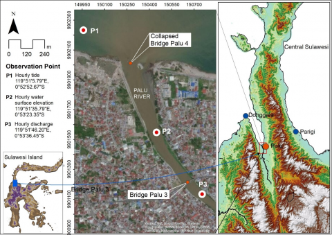
Approximately 1,000 m of the downstream segment of the Palu River around the estuary is the site of this research. This segment is located at the southern end of Palu Bay, Palu City, Sulawesi, Indonesia (Figure 1), one of the areas affected by the earthquake and tsunami on 28 September 2018. In addition to damaging the coastal area along the Palu Bay, the tsunami has also collapsed the Palu 4 bridge, the longest bridge on the Palu River (Figure 1). The selection of this site was based on several aspects, including: availability of DEMNAS data, flow data and strategic considerations of the location. This segment is considered important due to the complexity of community activities at the mouth of the river and the intensity of bed morphology changes due to interference between river flow and tides.
2.2 Data details
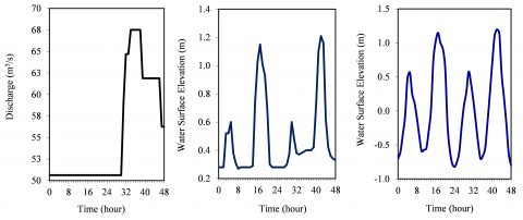
The main data assigned in this study are geometric data, tidal data, water level data, discharge data, and other related data. Geometric data is sourced from terrestrial surveys and BIG [8]. Both of these data are related to the formation of geometry in the 2D model. The next three data were obtained from direct observations at P1, P2 and P3 (Figure 1) at the same time, which were applied as the input to the boundary. These observation data were measured every hour for two days from 17 to 18 March 2021. The discharge and tidal data at the two observation points are shown in Figure 2a and Figure 2c, while the water level data for controlling the model is presented in Figure 2.
2.3 2D hydrodynamic model
The hydrodynamic simulation is performed based on the Resource Management Associates Module 2 (RMA2) developed by the United States Army Corps of Engineers (USACE). This 2D module is generally applied to simulate flows in rivers and beaches consisting of currents and water levels in both subcritical and supercritical conditions. The finite element method of the Galerkin scheme is applied to solve the differential equations in this model, which is initiated by discretizing the computational domain into a number of smaller sub-domains (elements). The basic equation of this model follows the governing equation derived from the Navier-Stokes Equation as follows [14, 15]:
$\frac{\partial h}{\partial t}+h\left(\frac{\partial u}{\partial x}+\frac{\partial v}{\partial y}\right)+u \frac{\partial h}{\partial x}+v \frac{\partial h}{\partial y}=0$ (1)
where, h is the water depth (m) and u and v are the velocity in the x and y directions (m/s).
Figure 1. Site map of the study area where situated at the downstream reach of Palu River, Central Sulawesi Indonesia
(a) (b) (c)
Figure 2. Observation data for two days on March 17th – 18th, 2021: (a) hourly discharge at the upstream of Bride Palu 3, (b) hourly water surface elevation at P2, (c) hourly tidal of Palu Estuary after correcting with MSL
2.4 Methods
The hydrodynamic simulation was performed in two scenarios. The first scenario is based on the geometry formed from terrestrial survey data. The upstream and downstream boundary conditions were inputted with the data as shown in Figure 2a and Figure 2c. Parameter adjustments, especially roughness value and standard eddy velocity, are executed to obtain optimal performance, which is measured by efficiency of Nash–Sutcliffe (NSE):
$N S E=1-\frac{\sum_{t=1}^{n}\left(h_{s i m_{-}}^{t} \,\,h_{o b s}^{t}\right)^{2}}{\sum_{t=1}^{n}\left(h_{s i m}^{t}\,\,-\,\,\bar{h}_{o b s}\right)^{2}}$ (2)
where, $h_{s i m}^{t}, h_{o b s}^{t}$, and $\bar{h}_{o b s}$ are simulated, observed and the mean of observed water depths in meter. The NSE is a dimensionless parameter and it is grouped based on the model's performance criteria: very good (0.75<NSE$\leq$1.00), good (0.65<NSE$\leq$0.70), moderately good (0.50<NSE$\leq$0.65) and poor (NSE$\leq$0.65) [16].
The last scenario is implemented using DEMNAS geometry data. The similar procedure is applied as in the first scenario, both on the boundary conditions and model parameters. The simulated water level in this scenario is also compared with the observed water level by referring to the NSE.
3.1 Geometry mesh and bed elevation
Mesh is the basis for constructing 2D geometries to solve finite difference numerical in the RMA2 model. The mesh can be in the shape of a triangle or quadrilateral depending on the complexity of the domain, especially the irregularity of domain boundaries and bed elevation. The mesh size is also greatly influenced by these two factors. In low-sloping bed topography, the mesh size can be larger than at high-slope.
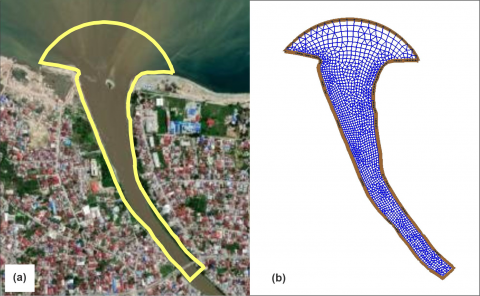
The boundary of the model domain in this paper is as in Figure 3a starting from the downstream of the river mouth to the upstream of the Bridge Palu 3. This segment is a tidal affected area due to the low elevation of the river bed below MSL. Semi-diurnal tide fluctuations continuously have an impact on progressive bed morphological changes along the segment.
The number of mesh elements of the domain is very important in this 2D simulation. The coverage area also determines the number of elements, but the number of these elements is usually very dependent on user assumptions such as the number and distance of nodes at domain boundaries. This is related to the numerical stability of the simulation process. The number of meshes in this study is 1879 elements (Figure 3b).
Figure 3b also provides information about mesh density. The upstream mesh tends to be denser than the downstream mesh as the bed slope decreases. At the domain boundary, the mesh density also tends to be higher, except at the downstream boundary. The density of the mesh is proportional to the number of elements per unit area and it also affects the stability of the computation.
In some cases, the mesh shape is generally non-uniform. By default, the geometry will be formed according to the initial settings when converting the map to a 2D mesh. The element shape conversion can be done automatically, and if the user feels the element shape still doesn't match the selected feature, then the element conversion can be done manually.
Figure 3. Detail of the study area: (a). boundary and (b) mesh
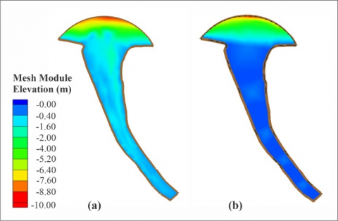
Figure 4. Bed elevation of the simulation domain generated from data of: (a). terrestrial survey and (b) DEMNAS
Figure 3b also shows a non-uniform mesh shape in almost all domains. Some elements have been converted to meet numerical stability especially in the upstream where the base elevation can change drastically due to deposition. The shape and density of this mesh can be evaluated at any time before the numerical simulation is performed. However, this initial evaluation has not been able to guarantee that the running model can run well.
Figure 4 presents the bed elevation for each node element. Elevation variability appears to be higher in Figure 4a than in Figure 4b across the domains. The source of the bed elevation in Figure 4a is a terrestrial survey using theodolite, water pass and echo-sounder. The first two instruments were applied to the shallow water area on the river side and in the deep-water area on the sea side, the survey was executed using an echo-sounder.
Figure 4b shows the low variation of depth especially on the river side. The variation of depth on the sea side is almost the same as Figure 4a, where the bottom depth changes gradually towards the sea at elevation intervals of -2 m to -10 m. The data for this elevation visualization is derived from DEMNAS and equipped with National Bathymetry data on the sea side.
3.2 Simulation performance based on the two types of geometry data
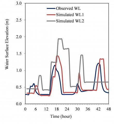
The hydrodynamic simulation has been performed based on two geometric conditions as mentioned in the previous section. The boundary conditions for both simulations were set the same type and time: hourly discharge and tide for 48 hours. The first simulation is designed to determine the most optimal geometric physical parameters with reference to the NSE by assessing the difference between the observed and simulated water levels at P2. Automatic parameter calibration cannot be carried out in the RMA2 Model, so the trial method is applied repeatedly. A number of simulation repetitions have been run and the highest performance was obtained at the NSE of 0.58 (Table 1).
With reference to the NSE goodness scale, the performance of this simulation scenario is quite good. More similar curves can be found in the low tide period compared to the high tide period (Figure 5). This illustrates that water level fluctuations under unsteady conditions are a very complex phenomenon. The limitations of the model often cannot accommodate this complexity [17]. However, the largest factor that affects the simulation performance is the geometric characteristics which include the suitability of the shape and the roughness of the bed material [18].
Table 1. NSE of simulated water level at Point 2
|
Water Level (m) |
NSE Calculation |
|||||
|
Time (hour) |
Observed (Hobs) |
Simulated 1 (Hsim-1) |
Simulated 2 (Hsim-2) |
(Hobs - Hobs-av)2 |
(Hobs - Hsim-1)2 |
(Hobs - Hsim-2)2 |
|
1 |
0.28 |
0.32 |
0.45 |
0.04 |
0.00 |
0.03 |
|
2 |
0.28 |
0.32 |
0.45 |
0.04 |
0.00 |
0.03 |
|
3 |
0.28 |
0.32 |
0.45 |
0.04 |
0.00 |
0.03 |
|
4 |
0.52 |
0.32 |
0.45 |
0.00 |
0.04 |
0.00 |
|
5 |
0.52 |
0.32 |
0.45 |
0.00 |
0.04 |
0.00 |
|
6 |
0.60 |
0.54 |
0.45 |
0.01 |
0.00 |
0.02 |
|
7 |
0.38 |
0.50 |
0.45 |
0.01 |
0.01 |
0.00 |
|
8 |
0.31 |
0.30 |
0.83 |
0.03 |
0.00 |
0.27 |
|
9 |
0.27 |
0.25 |
0.83 |
0.05 |
0.00 |
0.31 |
|
10 |
0.28 |
0.25 |
0.42 |
0.04 |
0.00 |
0.02 |
|
11 |
0.28 |
0.25 |
0.42 |
0.04 |
0.00 |
0.02 |
|
12 |
0.28 |
0.25 |
0.42 |
0.04 |
0.00 |
0.02 |
|
13 |
0.28 |
0.25 |
0.42 |
0.04 |
0.00 |
0.02 |
|
14 |
0.28 |
0.25 |
0.42 |
0.04 |
0.00 |
0.02 |
|
15 |
0.29 |
0.44 |
1.24 |
0.04 |
0.02 |
0.90 |
|
16 |
0.75 |
0.81 |
1.24 |
0.07 |
0.00 |
0.24 |
|
... |
... |
... |
... |
... |
... |
... |
|
... |
... |
... |
... |
... |
... |
... |
|
... |
... |
... |
... |
... |
... |
... |
|
42 |
1.10 |
0.85 |
0.65 |
0.37 |
0.06 |
0.20 |
|
43 |
1.21 |
1.33 |
0.65 |
0.52 |
0.01 |
0.31 |
|
44 |
1.16 |
1.33 |
0.65 |
0.45 |
0.03 |
0.26 |
|
45 |
0.62 |
1.33 |
0.65 |
0.02 |
0.50 |
0.00 |
|
46 |
0.42 |
0.62 |
0.65 |
0.00 |
0.04 |
0.05 |
|
47 |
0.36 |
0.44 |
0.65 |
0.02 |
0.01 |
0.08 |
|
48 |
0.34 |
0.44 |
0.65 |
0.02 |
0.01 |
0.10 |
|
Average (av) |
0.49 |
Total |
3.69 |
1.54 |
16.57 |
|
|
|
NSE |
0.58 |
-3.49 |
|||
Figure 5. Water surface elevation at P2 during time observation and simulations
The second simulation has also been executed to assess the performance of the model based on geometry sourced from terrestrial survey data combined with bathymetric data. Figure 5 shows the graph of this simulation result, where the difference in the trend of the two curves is very large. This shows that the performance of the model with this geometry is very low and it is confirmed by the negative NSE value of -3.49 (Table 1). This NSE illustrates that DEMNAS data has not been able to describe the bottom topography of the waters. Spatial resolution, especially vertical resolution, must be improved.
3.3 Water depth and water surface elevation
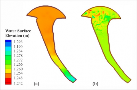
Both simulation results can be visualized with water surface elevation and water depth in the entire domain at maximum conditions as shown Figure 6 and Figure 7. The two figures are related to each other.
Figure 6. Water surface elevation resulting from hydrodynamic simulations over the entire domain: (a). terrestrial survey (b) DEMNAS
The water depth and water surface elevation in Figure 6a and Figure 7b are in line with the base elevation in Figure 4, where this geometry is formed from terrestrial survey data. The results of this simulation have confirmed previous studies that terrestrial survey data and high resolution DEM data generate a good performance of simulation results [19-21]. However, different things are shown in Figures 6b and 7b, water depth and water surface elevation do not confirm bed elevation in Figure 4. This also supports NSE in Table 1 that DEMNAS data has not given satisfactory results, as in line with the publications presented by Laks et al. (2017) [22].
Figure 7. Water depth resulting from hydrodynamic simulations over the entire domain: (a). terrestrial survey (b) DEMNAS
2D hydrodynamic simulation has been carried out in the downstream segment of the Palu River, Central Sulawesi Province, Indonesia. This simulation is based on domain geometry generated from two different types of data, namely terrestrial survey data and National DEM data (DEMNAS). Terrestrial survey data was obtained from direct investigations at the study site and DEMNAS data was derived from the Geospatial Information Agency of Indonesia. Both data were applied to create the mesh geometry of the modeled area.
Both simulation scenarios are performed with similar input conditions, roughness value, and standard eddy velocity method. The simulation results show that the model's performance is quite good with an NSE of 0.58 for terrestrial survey data geometry. On the contrary, poor performance is given by the simulation based on DEMNAS geometry with NSE of -3.49. This implies that for the case in this area, DEMNAS data still cannot be used to form a mesh model. This may be due to the insufficient vertical resolution of the DEM data even though the horizontal resolution is quite good. In addition, the modeled area is a low-sloping topography so that a better vertical resolution of the DEM is needed. However, the simulation performance needs to be tested on the upstream section or on the moderate to high slope river segment using geometries with similar DEMs resolution.
This research was funded by Graduate Program, Universitas Tadulako with Grant Number: 3013/UN28.2/KP/2021, March 23rd, 2021. Authors thank the director of graduate program for supporting this work through DIPA Pascasarjana Research Competition.
|
h |
the water depth, m |
|
u |
the velocity in the x directions, m. s-1 |
|
v |
the velocity in the y directions, m. s-1 |
|
x |
horizontal axis |
|
y |
vertical axis |
|
BIG |
Indonesian geospatial information agency |
|
DEMNAS |
national DEM |
|
MSL |
mean sea level |
|
NSE |
efficiency of Nash–Sutcliffe |
|
RMA2 |
resource management associates module 2 |
|
2D |
two dimensional |
|
P1 |
Point 1 |
|
P2 |
Point 2 |
|
P3 |
Point 3 |
|
Greek symbols |
|
|
$\partial$ |
partial differential operator |
|
Subscripts |
|
|
t |
time, hour |
|
obs |
observation |
|
sim |
simulation |
[1] Pramanik, N., Panda, R.K., Sen, D. (2010). One dimensional hydrodynamic modeling of river flow using DEM extracted river cross-sections. Water Resources Management, 24: 835-852. https://doi.org/10.1007/s11269-009-9474-6
[2] Ifiginia, Pudyastuti, P.S., Kuswartomo, Hidayati, N. (2018). The analysis of backwater impact on the increasing of floodwater level in Palu River. AIP Conference Proceedings, 1977(1): 050007. https://doi.org/10.1063/1.5043011
[3] Sabhan, Koropitan, A.F., Purba, M., Pranowo, W.S. (2019). 3D simulation model of tidal, internal mixing and turbulent kinetic energy of Palu Bay. Nature Environment and Pollution Technology, 18(4): 1083-1094.
[4] Pasternack, G.B., Wang, C.L, Merz, J.E. (2004). Application of a 2D hydrodynamic model to design of reach-scale spawning gravel replenishment on the Mokelumne River, California. River Research and Applications, River Research and Applications, 20(2): 205-225. https://doi.org/10.1002/rra.748
[5] Vaze, J., Teng, J., Spencer, G. (2010). Impact of DEM accuracy and resolution on topographic indices. Environmental Modelling & Software, 25(10): 1086-1098. https://doi.org/10.1016/j.envsoft.2010.03.014
[6] Zhu, D., Ren, Q., Xuan, Y., Chen, Y., Cluckie, I.D. (2013). An effective depression filling algorithm for DEM-based 2-D surface flow modelling. Hydrology and Earth System Sciences, 17(2): 495-505. https://doi.org/10.5194/hess-17-495-2013
[7] Sandbach, S.D., Nicholas, A.P., Ashworth, P.J., Best, J.L., Keevil, C.E., Parsons, D.R., Prokocki, E.W., Simpson, C.J. (2018). Hydrodynamic modelling of tidal-fluvial flows in a large river estuary. Estuarine, Coastal and Shelf Science, 212: 76-188. https://doi.org/10.1016/j.ecss.2018.06.023
[8] Geospatial Information Agency. (2021). National DEM (DEMNAS). http://tides.big.go.id/DEMNAS/, accessed on 15 August 2021.
[9] Tunas, I.G. (2019). The Application of ITS-2 Model for flood hydrograph simulation in large-size rainforest watershed, Indonesia. Journal of Ecological Engineering, 20(7): 112-125. https://doi.org/10.12911/22998993/109882
[10] Mandlburger, G., Hauer, C., Höfle, B., Habersack, H., Pfeifer, N. (2009). Optimisation of LIDAR derived terrain models for river flow modelling. Hydrology and Earth System Sciences, 13(8): 1453-1466. https://doi.org/10.5194/hess-13-1453-2009
[11] Shen, D., Wang, J., Cheng, X., Rui, Y., Ye, S. (2015). Integration of 2-D hydraulic model and high-resolution lidar-derived DEM for floodplain flow modeling. Hydrology and Earth System Sciences, 19(8): 3605-3616. https://doi.org/10.5194/hess-19-3605-2015
[12] Tunas, I.G., Maadji, R. (2018). The use of GIS and hydrodynamic model for performance evaluation of flood control structure. International Journal on Advanced Science, Engineering and Information Technology, 8(6): 2413-2420. http://dx.doi.org/10.18517/ijaseit.8.6.7489
[13] Li, J., Zhao, Y., Bates, P., Neal, J., Tooth, S., Hawker, L., Maffei, C. (2020). Digital elevation models for topographic characterisation and flood flow modelling along low-gradient, terminal dryland rivers: A comparison of spaceborne datasets for the Río Colorado, Bolivia. Journal of Hydrology, 591: 125617. https://doi.org/10.1016/j.jhydrol.2020.125617
[14] Park, S.W., Ahn, J. (2019). Experimental and numerical investigations of primary flow patterns and mixing in laboratory meandering channel. Smart Water, 4(4): 1-15. https://doi.org/10.1186/s40713-019-0016-y
[15] Xie, Q.J., Su, H., Chen, Z.J., Chen, J.J. (2015). Numerical simulation of the hydrodynamics of Jinshan Lake affected by strong wind. Journal of Yangtze River Scientific Research Institute, 32(4): 55-58. https://doi.org/10.3969/j.issn.1001-5485.2015.04.011
[16] Moriasi, D.N., Arnold, J.G., van Liew, M.W., Bingner, R.L, Harmel, R.D., Veith, T.L. (2007). Model evaluation guidelines for systematic quantification of accuracy in watershed simulations. Transactions of the American Society of Agricultural and Biological Engineers, 50(3): 885-900. https://doi.org/10.13031/2013.23153
[17] Costabile, P., Macchione, F., Natale, L., Petaccia, G. (2015). Flood mapping using LIDAR DEM. Limitations of the 1-D modeling highlighted by the 2-D approach. Natural Hazards, 77: 181-204. https://doi.org/10.1007/s11069-015-1606-0
[18] Conner, J.T., Tonina, D. (2014). Effect of cross‐section interpolated bathymetry on 2D hydrodynamic model results in a large river. Earth Surface Processes Landforms, 39(4): 463-475. https://doi.org/10.1002/esp.3458
[19] Gichamo, T.Z., Popescu, I., Jonoski, A., Solomatine, D. (2012). River cross-section extraction from the ASTER Global DEM for flood modeling. Environmental Modelling & Software, 31: 37-46. https://doi.org/10.1016/j.envsoft.2011.12.003
[20] Kang, C., Chan, D. (2018). Numerical simulation of 2D granular flow entrainment using DEM. Granular Matter, 20(13): 2-17. https://doi.org/10.1007/s10035-017-0782-x
[21] Tarekegn, T.H., Haile, A.T., Rientjes, T., Reggiani, P., Alkema, D. (2020). Assessment of an ASTER-generated DEM for 2D hydrodynamic flood modeling. International Journal of Applied Earth Observation and Geoinformation, 12(6): 457-465. https://doi.org/10.1016/j.jag.2010.05.007
[22] Laks, I., Sojka, M., Walczak, Z., Wróżyński, R. (2017). Possibilities of using low quality digital elevation models of floodplains in hydraulic numerical models. Water, 9(4): 1-19. https://doi.org/10.3390/w9040283