Silvia Luciani | Gianluca Coccia* | Sebastiano Tomassetti | Mariano Pierantozzi | Giovanni Di Nicola
OPEN ACCESS
The comparison between I-V (current-voltage) curves measured on site and I-V curves declared by the manufacturer allows to detect decrease of performance and control the degradation of photovoltaic modules and strings. On site, I-V curves are usually obtained under operating conditions (OPCs), i.e. at variable solar radiation and module temperature. OPC curves must be translated into standard test conditions (STCs), at a global irradiance of 1000 W/m2 and a module temperature of 25 °C. The correction at STC conditions allows to estimate the deviation between the power of the examined module and the maximum power declared by the manufacturer. A possible translation procedure requires two correction parameters: Rs’, the internal series resistance, and k’, the corresponding temperature coefficient. The aim of this work is to determine the correction parameters carrying out specific experimental tests as indicated by IEC 60891. A set of brand-new photovoltaic modules was experimentally characterized determining their I-V curves by means of an indoor solar flash test device based on a class A+ AM 1.5 solar simulator. Using the OPC I-V curves, obtained at several conditions of irradiance and temperature, it was possible to determine the correction parameters of the photovoltaic modules being considered.
PV modules, experimental, solar simulator, correction parameters, flash test
I-V (current-voltage) curves are an important tool to estimate the performance of photovoltaic (PV) modules and strings. In fact, during their lifetime, the components of PV plants can be subject to degradation, and this leads to loss of power and consequent decrease of expected production [1]. The comparison between I-V curves measured on site and I-V curves declared by the manufacturers offers the possibility to control the degradation of PV systems and detect decreases of performance.
On site, I-V curves can be obtained by means of commercial I-V curve tracers, which work according to the international standard IEC 60891 [2]. Since the operating conditions (OPCs) of PV modules do not generally coincide with the standard conditions (STCs), which consider a global irradiance (G) equal to 1000 W/m2 and a temperature (T) of the module of 25°C, I-V curves need to be translated. Only with this correction it is possible to compare the deviation between the power measured in the examined module and the maximum power declared by the manufacturer.
Based on the standard IEC 60891, three correction procedures can be used to translate OPC curves into STC curves. Commercial I-V curve tracers usually follow the second procedure proposed by the standard, which requires two correction parameters: Rs’, the internal series resistance of the test specimen, and k’, that can be interpreted as the temperature coefficient of the internal series resistance Rs’. The second procedure also considers an additional parameter a, defined as the irradiance correction factor for open circuit voltage; the standard IEC 60891 suggests a value of 0.06 for a, if no additional data are available. According to the IEC 60891, the correction parameters can be determined by means of specific experimental procedures, with natural sunlight or with a solar simulator able to carry out flash tests.
As outlined by the authors in a previous publication [3], in the technical literature a systematic evaluation of the correction parameters is difficult to be found. Therefore, it is not an easy task to find reference values for Rs’ and k’. It should be noted that the two correction parameters are not provided both by manufacturers in the datasheets of PV modules and by the software of commercial I-V curve tracers; without the coefficient parameters, it is thus impossible to check the accuracy of the STC I-V translation carried out by a curve tracer and there is no possibility to determine STC translations with other systems. For this reason, we believe that an analysis focused on the experimental determination of the two parameters could be of academic and technical interest. In the following, we will summarize some of the main contributions that can be found in literature about correction procedures for I-V curves of PV modules.
In 2010, Paghasian [4] applied the correction procedures reported in IEC 60891 to PV modules of different technology, and found the following values for Rs’, k’ and a, respectively: (0.5 Ω, -0.045 Ω.°C-1, -0.075) for Si-based monocrystalline cells, (-17 Ω, -0.09 Ω.°C-1, -0.0095) for Si-based amorphous cells, (1.5 Ω, -0.7 Ω.°C-1, -0.1) for CdTe-based cells, and (2.85 Ω, -0.005 Ω.°C-1, -0.06) for CIGS-based cells. To obtain data at different irradiance levels, various mesh screens with changing light transmittance were used; on the other hand, to obtain data at different temperatures, the tested modules were pre-cooled in an air-conditioned wooden cabinet or an environmental chamber. The I-V curves were performed under sunlight while the modules warmed up in natural way.
In a successive work, Paghasian and TamizhMani [5] considered four correction procedures (three from IEC 60891 and one from NREL) and evaluated their accuracy. The correction parameters were determined with natural sunlight for the same technologies described above: mono-Si, a-Si, CdTe, and CIGS. The I-V curves of the modules were evaluated at different temperatures, by pre-cooling them and then allowing them to warm up naturally under solar radiation. In addition, mesh screens of varying light transmittance were used to evaluate the performance of the modules at different irradiation values.
In 2011, Abella and Chenlo [6] used a class AAA solar simulator to determine the temperature coefficients and the correction parameters of several Si-based polycrystalline cells PV modules, extrapolating these data from the I-V curves. Tests were carried out at temperatures ranging from 20 to 50°C for a fixed irradiance of 1000 W/m², and at irradiances ranging from 700 to 1200 W/m2 for a fixed temperature of 25°C. The former tests allowed to the determine the parameters k and k’, which refer, respectively, to the correction procedures 1 and 2 reported in the IEC 60891. The authors found that the value of k that allowed to obtain the minimum dispersion of the maximum power (0.5%) was 0.0039 Ω.°C-1, while the value of k’ that allowed to obtain the minimum dispersion of the maximum power (0.4%) was 0.00345 Ω.°C-1. Instead, the tests carried out at a fixed temperature allowed to evaluate the parameters Rs and Rs’, for procedure 1 and 2, respectively. It was found that the value of Rs that gave the minimum dispersion of maximum power (0.4%) was 0.36 Ω, while the value of Rs’ that gave the minimum dispersion of power was 0.35 Ω.
In 2015, a systematic procedure was described by Dubey et al. [7] to measure temperature coefficients of PV modules in the field. The authors analyzed temperature coefficients for three modules of different PV technology (mono c-Si, multi c-Si and CIGS), and the coefficients were then compared to the values obtained by means of an indoor test rig. The temperature coefficient of voltage found for mono c-Si modules from field measurements was -0.31 %/°C, value that is similar to the one obtained with the indoor test rig, equal to -0.28%/°C. For the other two technologies, similar results were confirmed: for c-Si, -0.27%/°C in the field and -0.30%/°C in laboratory; for CIGS, 0.28%/°C in the field and -0.27%/°C indoor. For the same PV panels, the authors also measured the temperature coefficients of current; in this case, larger deviations were detected. The temperature coefficient of current for mono c-Si modules was found to be 0.021%/°C in the field and 0.03%/°C in laboratory; for multi c-Si modules, the temperature coefficient of current measured in the field was 0.026%/°C and 0.028%/°C in laboratory; for CIGS modules, the coefficient was determined to be 0.0029 %/°C in the field and 0.003%/°C in laboratory.
In 2016, Trentadue et al. [8] determined the internal series resistance of several PV modules of different technology (Si-based crystalline, Si-based amorphous, CdTe and CIGS), following the standard IEC 60891. Three aspects were investigated by the authors to evaluate the overall uncertainty for the determination of the series resistance. The first aspect was the temperature variation of the PV modules, which was found to have a relevant influence on uncertainty (5%). The second aspect was electrical noise, which led to a variation of 5%. The third aspect was the repeatability of the solar simulators used for the tests: while an average repeatability value of 5% was determined for most of PV modules, variations up to 15% were detected for CIGS thin-film systems. According to the results of the experimentation, an overall uncertainty of ±10% was found for the series resistance of the modules.
Piliougine et al. [9] studied the variation of series resistance respect to the module temperature and defined an experimental methodology to estimate the temperature coefficient k. The results obtained in their work are based on outdoor measurements. The work also presents the results of a study concerning the suitability of the single diode model (SDM) or the double diode model (DDM) for estimating Rs and calculating k by means of a linear regression with a high coefficient of determination R2. By using the SDM, the estimation of k ranges between 1.19 and 1.74 mΩ/°C, with a mean value of 1.43 mΩ/°C. Using the DDM, a range for k from 0.89 to 1.34 mΩ/°C, with a mean value equal to 1.06 mΩ/°C, was obtained. As for the series resistance Rs, the SDM gave an estimated value ranging from a minimum of 262 mΩ to a maximum of 320 mΩ, with an average of 288 mΩ. Using the DDM, higher values were estimated, i.e. ranging from 345 mΩ to 395 mΩ with a mean equal to 374 mΩ.
Based on the considerations reported above and the analysis of the literature, it is possible to state that the experimental evaluation of correction parameters needs to be deepened and discussed. For this reason, in this work a set of brand-new PV modules was experimentally characterized determining their I-V curves by means of an indoor solar flash test device based on a class A+ AM 1.5 solar simulator. Through the OPC I-V curves, obtained at several conditions of irradiance and temperature, it was possible to determine the correction parameters of the PV modules under study, referring to the second procedure reported in the IEC 60891.
The paper is organized as follows. The technical specifications of the indoor solar flash test device, together with the specification of the PV modules considered, are provided in Section 2. Section 3 describes the experimental procedure followed to determine the two correction parameters, Rs’ and k’. Section 4 reports the results of the study, and their discussion. The conclusions of the work can be found in Section 5.
In the present work, tests were performed by means of an indoor solar flash test device based on a class A+ AM 1.5 solar simulator, made by BERGER Lichttechnik. The system consists of a pulsed solar simulator (PSS), a load and measuring device (pulsed solar load, PSL), an infrared (IR) detector, a Pt100 sensor, a computer with dedicated software for I-V curves acquisition, and a tower system (Figure 1).
The PSS includes a power generator and a lamella light source without optical elements for homogenous and reproducible illumination. The device meets all the requirements of IEC 60904-9 [10], while the construction of the lamella light source and the patented flash tube ensure lifetime conformity with this standard.
The PSL is a processor-controlled device with three channels, used for measuring and load simulation. It allows to determine the I-V curves of PV modules, according to IEC 60904-1 [11].
Figure 1. Solar flash test device
The IR detector is a contactless, infrared measuring system with external sensor head that allows the automatic module temperature acquisition. The Pt100 sensor, instead, is a resistance temperature detector allowing the ambient and cell temperature acquisition.
Through the PSL software, installed in the dedicated computer, all relevant data relative to the I-V curves are acquired, stored and displayed. The tower system provides a stable test environment for improved uniformity and testing repeatability.
For the determination of the correction parameters, a specific dataset of three brand-new PV modules was selected. The modules belong to the same brand and have the same nominal power (345 W). They are characterized by 72 series-connected cells in polycrystalline silicon and consist of cell arrays, each with 24 cells in series and one bypass diode per cell array in parallel. The main parameters of the PV modules can be found in Table 1 and Table 2.
Table 1. Electrical characteristics of the PV modules
|
Parameter |
Symbol |
Value |
|
Maximum power |
Pmax (W) |
345 |
|
Current at maximum power point |
Impp (A) |
9.10 |
|
Voltage at maximum power point |
Vmpp (V) |
37.93 |
|
Short circuit current |
Isc (A) |
9.59 |
|
Open circuit voltage |
Voc (V) |
46.58 |
|
Maximum system voltage |
(V) |
1500 |
|
Module efficiency |
Eff (%) |
17.30 |
Standard test conditions: irradiance 1000 W/m², temperature 25°C +/- 2°C, AM 1.5.
The experimental method for the determination of Rs’, as indicated in the IEC 60891, requires that the current-voltage characteristics are traced at several irradiances and at constant temperature. For the purpose of changing irradiance, four metallic grids were used. Each grid is characterized by a different mesh width in mm, to guarantee a different useful surface for the passage of sunlight. The main characteristics of the grids can be found in Table 3.
Table 2. Thermal characteristics of the PV modules
|
Parameter |
Symbol |
Value |
|
Maximum power temperature coefficient |
g (%/°C) |
-0.40 |
|
Open circuit voltage temperature coefficient |
β (%/°C) |
-0.29 |
|
Short circuit current temperature coefficient |
α (%/°C) |
0.04 |
|
Nominal operating cell temperature |
NOCT (°C) |
43+/-3 |
|
Temperature range |
(°C) |
– 40 to 85 |
Standard test conditions: irradiance 1000 W/m², temperature 25°C +/-2°C, AM 1.5.
Table 3. Characteristics of the metal grids
|
Grid type |
Mesh width (mm) |
Useful surface for sunlight passage (%) |
|
AISI 304 L NF 55 |
0.395 |
61.17 |
|
AISI 304 L NF 70 |
0.297 |
55.96 |
|
AISI 304 L NF 90 |
0.209 |
45.77 |
|
AISI 304 L NF 120 |
0.132 |
32.33 |
On-site, I-V curves are being measured in provided operating conditions (OPCs), and they must be therefore translated into standard test conditions (STCs) to obtain measures independent of actual on-site temperature and irradiance. The international standard IEC 60891 defines three different correction procedures. It also defines the procedures used to determine the parameters relevant for these corrections.
The first procedure is equal to the procedure given in the first edition of the IEC 60891, but the equation has been rewritten for easier understanding. The second procedure is an alternative algebraic correction method which yields better results for large irradiance corrections (>20%). The two procedures require the correction parameters of the PV device to be known. If the parameters are not known, they need to be determined before performing the correction. The third procedure is an interpolation method that does not require correction parameters as input: it can be applied when a minimum of three I-V curves have been measured for the test device. These three I-V curves span the temperature and irradiance range for which the correction method is applicable.
The first correction procedure requires that the measured I-V curves shall be corrected to standard test conditions or other selected temperature and irradiance conditions by applying the following equations:
$I_{2}=I_{1}+I_{\mathrm{sc}} \cdot\left(\frac{G_{2}}{G_{1}}-1\right)+\alpha \cdot\left(T_{2-} T_{1}\right)$ (1)
and
$V_{2}=V_{1}-R_{S} \cdot\left(I_{2-} I_{1}\right)-k \cdot I_{2} \cdot\left(T_{2-} T_{1}\right)+ \beta\cdot\left(T_{2-} T_{1}\right)$ (2)
where:
The second correction procedure is based on the simplified one-diode model of PV devices. It is defined by the following equations for current and voltage, respectively:
$I_{2}=I_{1}\left[1+\alpha_{\mathrm{rel}}\left(T_{2-} T_{1}\right)\right] \frac{G_{2}}{G_{1}}$ (3)
and
$\begin{aligned} V_{2}=V_{1} &+V_{\mathrm{oc} 1}\left[\beta_{\mathrm{rel}}\left(T_{2-} T_{1}\right)+a \ln \left(\frac{G_{2}}{G_{1}}\right)\right] \\ &-R_{\mathrm{s}}^{\prime}\left(I_{2-} I_{1}\right)-k^{\prime} I_{2}\left(T_{2-} T_{1}\right) \end{aligned}$ (4)
where:
The third correction procedure is based on the linear interpolation or extrapolation of two measured I-V curves. The measured I-V characteristics shall be corrected to STC or other selected temperature and irradiance values by applying the following equations:
$V_{3}=V_{1}+a \cdot\left(V_{2}-V_{1}\right)$ (5)
and
$I_{3}=I_{1}+a \cdot\left(I_{2}-I_{1}\right)$ (6)
The pair of points (I1, V1) and (I2, V2) should be selected so that I2 - I1 = Isc2 – Isc1, where:
$G_{3}=G_{1}+a \cdot\left(G_{2}-G_{1}\right)$ (7)
$T_{3}=T_{1}+a \cdot\left(T_{2}-T_{1}\right)$ (8)
Since most of commercial I-V curve tracers follows the second correction procedure, only this method will be analyzed in the following. From Eqns. (3) and (4), it can be seen that, besides the temperature coefficients for short circuit current αrel and open circuit voltage βrel, generally indicated in the module datasheet, other three correction parameters have to be defined to perform the correction procedure from OPC to STC conditions: a, Rs’ and k’. While IEC 60891 indicates for a a typical value of 0.06, no reference values can be found for Rs’ and k’, which should be determined experimentally (in natural or simulated sunlight).
IEC 60891 defines the experimental methods to determine Rs’ and k’ in natural sunlight or simulated sunlight according to two different steps. In the first step, experimental tests are performed to determine a and Rs’. To perform the flash tests at different irradiations and at constant temperature, four different metallic grids were placed on the modules. As described above, the four metallic grids are characterized by a different mesh width in mm, such as to guarantee a different useful surface for the passage of the sunlight with an emitted radiation reduction. To determine all the I-V curves, each of the three modules was placed on a dedicated support inside the tower system and was placed underneath the flasher, connected to the PSS. For the first module, the following measurement phases were performed at constant temperature:
The same procedure was repeated for the other two modules.
In the second step, experimental tests are performed to determine k’. In this phase, flash-tests are carried out at constant irradiance but at different temperatures. To determine all the I-V curves, each of the three modules was placed on a dedicated support inside the tower system and was placed underneath the flasher, connected to the PSS. For the first module, the following measurement phases were performed at constant irradiance:
Even in this case, the procedure was repeated for the other two PV modules.
This section presents and discusses the results of the experimental measurements. Considering the first PV module as a reference, the determination of Rs’ was accomplished according to the following steps.
Five I-V curves were first traced at constant temperature and at five different irradiances. The curves are reported in the diagram of Figure 2.
Figure 2. I-V curves measured at different irradiances and constant temperature (module 737)
Assuming that Isc1 is the short-circuit current of the I-V characteristic recorded at highest irradiance G1, equal to 1234.98 W/m², we translated sequentially all the other four curves recorded at lower irradiances to G1, using Rs’ = 0 Ω and a = 0 as starting values with Eqns. (3) and (4). We plotted the corrected I-V curves in another diagram (Figure 3).
Figure 3. I-V curves corrected at a = 0 and Rs’ = 0 Ω (module 737)
Then, we increased the parameter a of Eq. (4) with steps of 0.001, maintaining the condition Rs’ = 0 Ω. The proper value of a was determined when the open circuit voltages of the transposed I-V characteristics coincided within 0.5% or better (Figure 4). The final value found for a was equal to 0.048.
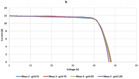
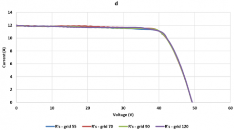
With the value a = 0.048, we thus used the relation ns/np x 10 mΩ as an estimate for the internal series resistance Rs’, where ns is the number of cells connected in series and np is the number of parallel connected blocks in the PV module. For the tested modules, ns is equal to 24 and np is equal to 3. Then, we changed Rs’ in steps of 10 mΩ in the positive direction, and the proper value of Rs’ was determined when the deviation of the maximum output power values of the transposed I-V characteristics coincided within ±0.5% or better. The final value found for Rs’ was equal to 0.34 Ω (Figure 5).
Figure 4. I-V curves corrected at a = 0.048 and Rs’ = 0 Ω (module 737)
Figure 5. I-V curves corrected at a = 0.0048 and Rs’ = 0.34 Ω (module 737)
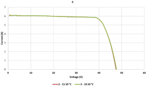
For the determination of k’, the temperature coefficient of the internal series resistance Rs’, the following steps were carried out. We first traced I-V curves at three different temperatures and at constant irradiance equal to 640 W/m² (Figure 6).
Figure 6. I-V curves measured at different temperatures and constant irradiance (module 737)
The lowest temperature T1 was equal to 10.80°C. Then, we translated sequentially the other two curves recorded at higher temperatures to T1, using k’ = 0 Ω/K in Eq. (4). The corrected I-V curves are provided in the diagram of Figure 7.
Figure 7. Temperature-corrected I-V curves with k’ = 0 Ω/K (module 737)
Starting from 0 mΩ/K, k’ was varied with steps of 1 mΩ/K in the positive direction. The proper value of k’ was determined when the deviation of the maximum output power values of the transposed I-V characteristics coincided within ± 0.5% (Figure 8). The final value found for k’ was equal to 0.009 Ω/K.
Figure 8. I-V curves corrected with k’ = 0.009 Ω/K
The procedures used to determine Rs’ and k’ for the first module were also applied to determine the same correction parameters in the other two modules. A summary of the correction parameters found for the three modules are provided in Table 4. It is possible to note that there is a consistency in the values found for k’, while the values assumed by a and Rs’ are more variable.
Table 4. Summary of a, Rs’, k’ for each PV module
|
Module serial number |
a (-) |
Rs’ (Ω) |
k’ (Ω/K) |
|
737 |
0.048 |
0.34 |
0.009 |
|
712 |
0.050 |
0.43 |
0.009 |
|
767 |
0.046 |
0.40 |
0.010 |
For the PV modules under study, Table 5 shows a comparison between the main electrical quantities determined with a commercial I-V curve tracer (which uses its default correction parameters) and the same quantities determined with the correction parameters found experimentally. As can been seen, all deviations are inferior than 1%; this can be considered a good validation of the experimental tests carried out to determine the correction parameters.
Table 5. Comparison of the main electrical parameters for the PV modules determined with the curve tracer (CT) and with the experimental correction parameters (exp)
|
Parameter/Module |
737 |
712 |
767 |
|
Voc (V) – CT Voc (V) – exp |
48.3 48.6 |
45.9 46.2 |
47.5 47.8 |
|
Isc (A) – CT Isc (A) - exp |
9.2 9.2 |
9.2 9.2 |
9.2 9.2 |
|
Vmpp (V) – CT Vmpp (V) – exp |
38.2 38.1 |
35.9 35.9 |
37.4 37.3 |
|
Impp (A) – CT Impp (A) – exp |
8.6 8.6 |
8.5 8.5 |
8.5 8.6 |
|
Pmax (W) – CT Pmax (W) – exp |
329.0 328.9 |
306.4 305.9 |
320.5 320.1 |
In this work, an experimental procedure was carried out to determine the correction parameters of a set of PV (photovoltaic) modules according to the standard IEC 60891. The PV modules were characterized by determining their I-V (current-tension) curves through an indoor solar flash test device based on a class A+ AM 1.5 solar simulator. The I-V curves were obtained at different conditions of temperature and irradiance.
Based on the results of the experimental analysis, the procedure suggested by the standard IEC 60891 allowed to determine the correction parameters within the maximum tolerance of 5%. In order to confirm the validity of the experimental procedure, the STC (standard test condition) I-V curves determined with the correction parameters were compared with those provided by a commercial curve tracer. In this case, deviations smaller than 1% were obtained; this result can be considered a good validation of the experimental tests.
The knowledge of the correction parameters is very useful, as it allows to evaluate the electrical performance of PV modules without using curve tracers, that generally do not declare the values of the internal corrections parameters used. With the correction parameters, it is also possible to build and validate mathematical models of PV systems, which allow to evaluate the performance of such energy devices without using experimental testing.
|
AM |
air mass |
|
a |
irradiance correction factor for the open circuit voltage |
|
Eff |
module efficiency, % |
|
G |
irradiance, W.m-2 |
|
I |
current intensity, A |
|
k |
temperature coefficient, Ω.°C-1 |
|
k’ |
temperature coefficient, Ω.°C-1 |
|
NOCT |
nominal operating cell temperature, °C |
|
n |
number of I-V points |
|
P |
electrical power, W |
|
R2 |
coefficient of determination |
|
Rs’ |
internal series resistance, Ω |
|
T |
temperature, °C |
|
V |
voltage, V |
|
Greek symbols |
|
|
$\alpha$ |
short circuit current temperature coefficient, %.K-1 |
|
$\beta$ |
open circuit voltage temperature coefficient, %.K-1 |
|
g |
maximum power temperature coefficient, %.K-1 |
|
Subscripts |
|
|
1 |
OPC (operating conditions) |
|
2 |
STC (standard test conditions) |
|
max |
maximum |
|
mpp |
maximum power point |
|
oc |
open circuit |
|
rel |
relative |
|
sc |
short circuit |
|
Acronyms |
|
|
CIGS |
copper indium gallium selenide |
|
DDM |
double diode model |
|
IR |
infrared |
|
NREL |
National Renewable Energy Laboratory |
|
OPC |
operating condition |
|
PSL |
pulsed solar load |
|
PSS |
pulsed solar simulator |
|
PV |
photovoltaic |
|
SDM |
single diode model |
|
STC |
standard test condition |
[1] Jordan, D.C., Silverman, T.J., Wohlgemuth, J.H., Kurtz, S.R., VanSant, K.T. (2017). Photovoltaic failure and degradation modes. Progress in Photovoltaics: Research and Applications, 25(4): 318-326. https://doi.org/10.1002/pip.2866
[2] International Electrotechnical Commission (2009). IEC 60891. Procedures for temperature and irradiance corrections to measured IV characteristics of crystalline silicon photovoltaic devices. Second edition.
[3] Luciani, S., Coccia, G., Tomassetti, S., Pierantozzi, M., and Di Nicola, G. (2020). Use of an indoor solar flash test device to evaluate production loss associated to specific defects on photovoltaic modules. Tecnica Italiana - Italian Journal of Engineering Science, 64(2-4): 167-172. https://doi.org/10.18280/ijdne.150504
[4] Paghasian, K. (2010). Power Rating of Photovoltaic Modules: Repeatability of Measurements and Validation of Translation Procedures. Arizona State University.
[5] Paghasian, K., TamizhMani, G. (2011). Photovoltaic module power rating per IEC 61853–1: A study under natural sunlight. 2011 37th IEEE Photovoltaic Specialists Conference, Seattle, WA, USA, pp. 002322-002327. https://doi.org/10.1109/PVSC.2011.6186418
[6] Abella, A.M., Chenlo, F. (2011). Determination in solar simulator of temperature coefficients and correction parameters of PV modules according to international standards. 2011 37th IEEE Photovoltaic Specialists Conference, Seattle, WA, USA, pp. 002225-002230. https://doi.org/10.1109/PVSC.2011.6186399
[7] Dubey, R., Batra, P., Chattopadhyay, S., Kottantharayil, A., Arora, B.M., Narasimhan, K.L., Vasi, J. (2015). Measurement of temperature coefficient of photovoltaic modules in field and comparison with laboratory measurements. 2015 IEEE 42nd Photovoltaic Specialist Conference (PVSC), New Orleans, LA, USA, pp. 1-5. https://doi.org/10.1109/PVSC.2015.7355852
[8] Trentadue, G., Pavanello, D., Salis, E., Field, M., Müllejans, H. (2016). Determination of internal series resistance of PV devices: repeatability and uncertainty. Measurement Science and Technology, 27(5): 055005. http://dx.doi.org/10.1088/0957-0233/27/5/055005
[9] Piliougine, M., Spagnuolo, G., and Sidrach-de-Cardona, M. (2020). Series resistance temperature sensitivity in degraded mono–crystalline silicon modules. Renewable Energy, 162: 677-684. https://doi.org/10.1016/j.renene.2020.08.026
[10] International Electrotechnical Commission. (2007). IEC 60904–9. Photovoltaic devices, Part 9.
[11] International Electrotechnical Commission. (2006). 60904-1, Photovoltaic Devices, Part 1: Measurement of Photovoltaic Current–Voltage Characteristics. International Electrotechnical Commission, Geneva, Switzerland. Ed, 2.