Gianluca Coccia* | Alice Mugnini | Lorenzo Romanucci | Fabio Polonara | Alessia Arteconi
OPEN ACCESS
A way to improve the performance of heat pumps lies in the possibility of adhering to Demand Response (DR) programs. DR consists of changes in electricity use of end users in response to changes in the electricity price over time. Taking advantage of the energy flexibility given by the end-use system, such as a building, it is possible to collect more electricity when its price is low, and to reduce its absorption when the price is high. In this work, a commercial air-to-water heat pump was experimentally characterized to assess its energy performance when managed with a DR program. A test rig based on a closed-loop system allowed to reproduce a thermal load in the condenser side. The thermal load was associated to the space heating demand of a virtual building, which was modeled with a resistance-capacitance thermal network. The DR program, based on a real-time pricing control strategy, managed the interaction between the closed-loop system and the virtual building, which was able to unlock its energy flexibility thanks to a variable indoor air setpoint temperature. Respect to a conventional control based on a fixed setpoint temperature, the DR-based configuration led to significant electrical energy and cost saving.
demand response, experimental, heat pump, energy flexibility, real-time pricing
A relevant part of the global electricity demand is used for the HVAC (Heating, Ventilation, and Air-Conditioning) sector, demand that is expected to rise up to 4000 TWh in 2050 [1]. Space heating and cooling of buildings are responsible for about 30–45% of the energy demand [2], and in the European residential sector, where the main consumption of energy includes hot water production and space heating, heat production is largely based on non-renewable sources, which are responsible of large emissions of greenhouse gases [3]. Since this practice is not sustainable, the European Performance of Building Directive (EPBD) [4] required a nearly-zero energy building (nZEB) standard for new buildings by 2021. This standard has led to a widespread diffusion of high-efficient energy systems in the household market, in particular heat pumps. The use of heat pumps is growing rapidly: for example, with a 12% increase reached in 2018, the European heat pump market has achieved double-digit growth for the fourth year in a row, and a doubling of the European heat pump market by 2024 is expected [5].
Heat pumps, as well as other energy systems such as refrigerators, air-conditioners, etc., can be considered as thermostatically controlled loads in buildings. On the other hand, the energy flexibility provided by buildings is paramount to mitigate the upcoming challenges of future power systems, as outlined by the working group of Annex 67 about energy flexible buildings [6]. For this reason, if managed together in a smart way, heat pumps and buildings can be used to modify the electric load without affecting the quality of the energy service [7].
Considered the aforementioned points, space heating and cooling in buildings is promising for the application of demand side management (DSM) strategies aimed at altering the electrical energy demand of the final user. DSM includes all the policies used to influence the customer’s energy curve, focusing on changing the shape of the load and thereby helping to optimize the whole power system from generation to delivery, to end use [7, 8]. DSM strategies can have different objectives, e.g.: peak shaving, valley filling, load shifting, energy conservation, and strategic load growth [7]. One of the most important aspects of DSM is related to the growing share of renewable energy sources (RESs) in the generation mix and consequently to the necessity of managing them due to their intermittent and unpredictable production.
A possible DSM strategy is represented by demand response (DR), which refers to changes in electricity use of end customers from their normal consumption patterns in response to changes in the electricity price over time [8]. Usually, two types of tariffs can be found in the market: time of use (TOU) tariffs, varying on the period of the day, and real-time pricing tariffs, that change with the electricity market price [9]. Based on the electricity price, the heat pump demand can be shifted with the aim of reducing electricity costs, improving the system performance, increasing RESs integration, or improving power system benefits.
Given this premise, it is clear that the study of the energy performance of heat pumps used to meet the hot water and space heating demands of buildings, when the latter are able to unlock their energy flexibility thanks to a DR strategy, is paramount. Thus, in this work a commercial air-to-water heat pump was experimentally characterized to evaluate its energy performance when managed with a DR program. A test rig based on a closed-loop system allowed to reproduce a thermal load in the condenser side. The thermal load was associated to the space heating demand of a virtual building, which was modeled with a resistance-capacitance thermal network. The DR program, based on a real-time pricing control strategy, managed the interaction between the closed-loop system and the virtual building, which was able to unlock its energy flexibility thanks to a variable indoor air setpoint temperature. The results obtained with the DR program, in terms of energy and cost saving as well as thermal comfort, were compared with those obtained with a conventional control based on a fixed setpoint temperature (baseline).
The paper is organized as follows. The experimental setup, that includes the heat pump, the thermal load and the acquisition system, is described in Section 2. Section 3 reports the details of the case study, and how the baseline and the DR program were defined. Section 4 reports the results of the study, and their discussion. The conclusions of the work can be found in Section 5.
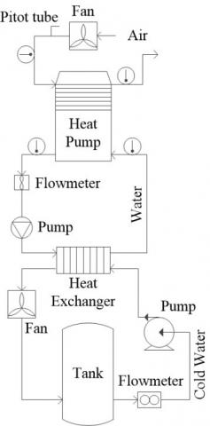
Figure 1. Test rig
The experimental setup (Figure 1) used to evaluate the effectiveness of the DR strategy consists of a commercial air-to-water heat pump (NIBE F370 3x400) and a dedicated test rig, installed at the DIISM (Department of Industrial Engineering and Mathematical Science). The heat pump has a nominal thermal power of 2 kWt and a nominal COP of 3.93, evaluated according to the standard EN 14511. The working refrigerant is propane (R290). The evaporator was realized by Luvata and is a compact heat exchanger with corrugated fins, 56 tube-passes and about 6 m2 of heat transfer surface. The fan that realizes the heat transfer between the air and the refrigerant has different setting speeds. The compressor of the heat pump is a scroll-type, with a nominal electrical power of 650 We. In the condenser side of the system, there is a pump that can be regulated with three different speeds. In the present study, the volumetric flow rate of water elaborated by the pump was around 8 L/min. The minimum and maximum supply temperatures of the heat transfer fluid were set to 50 and 55°C, respectively. Being a fixed-load heat pump, the two temperatures determine the ON and OFF cycles of the compressor.
In order to simulate the space heating load of a building, the water in the condenser side of the heat pump transfers heat to a countercurrent plate-and-frame heat exchanger, where the cold fluid is water collected from a dedicated tank. The electric pump that serves the cold-water side is controlled by an inverter, that works in the range 0-70 Hz; this allows a maximum rotational speed of 4200 RPM.
In the evaporator side of the heat pump, there are two T-type thermocouples that measure the inlet and outlet temperatures of air. A pitot tube allows to determine the air speed; the combination of the three sensors allows to evaluate the thermal power transferred from the air to the refrigerant. In a same fashion, in the condenser side of the heat pump there are two T-type thermocouples that measure the delivery and return temperatures of water. In the same circuit, there is also a turbine flowmeter that detects the volumetric flow rate of the heat transfer fluid. The knowledge of these quantities allows to estimate the thermal power transferred from the refrigerant to water. To determine the electrical power absorbed by the compressor and the other auxiliary devices of the heat pump, a power analyzer was installed between the system and the power grid. An electromagnetic flowmeter is also installed in the cold-water circuit, in order to measure the volumetric flow rate of the fluid elaborated by the electric pump. Additional thermocouples and pressure transducers are installed in the refrigerant circuit of the heat pump to evaluate the thermodynamic properties of the fluid in the main points of the reversed cycle.
All the measurement signals are acquired by means of a National Instruments cDAQ-9174 and processed with a dedicated LabVIEW virtual instrument. The cDAQ-9174 system includes three acquisition modules: 1) a NI 9214, that acquires the signals from the thermocouples; 2) a NI 9025, that manages the signals from the remaining sensors and transducers; 3) a NI 9263, that is used to send a voltage output signal to the inverter that controls the electric pump in the cold-water side.
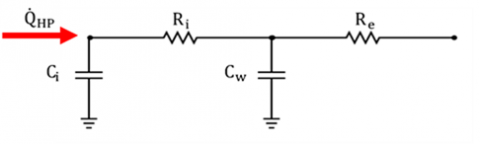
Figure 2. 2R2C resistance-capacitance thermal network of the virtual building
The case study considers that the heat pump is used to meet the space heating demand of a virtual building, which in the experimental setup described in Section 2 is simulated with the heat exchanger fed with cold water collected from the dedicated tank. In particular, two cases were evaluated: in the first case (referred to as baseline) the heat pump works with a fixed indoor air setpoint temperature, while in the second case (referred to as DR) the heat pump is allowed to work with a variable indoor air setpoint temperature, determined by means of a DR program based on a real-time pricing control strategy.
To simulate the thermal behavior of the virtual building, a simple 2R2C resistance-capacitance thermal network was used. As can be seen in Figure 2, this model assigns a capacitance (Ci) to the mass of air in the building, a capacitance (Cw) to the opaque walls of the envelope, a resistance (Ri) to the internal part of the opaque walls (all the layers from the internal surface up to the insulating material, which is not considered), and a resistance (Re) to the external part of the opaque walls (all the layers from the insulating material, which is included, up to the external surface). The model does not take into account the thermal behavior of transparent surfaces and it is assumed that the design space heating load is only by transmission through the walls. With these assumptions, the thermal behavior of the virtual building is described by the following set of two differential equations:
$\left\{\begin{array}{c}Q_{\mathrm{hp}}=\frac{T_{\mathrm{air}}-T_{\mathrm{w}}}{R_{\mathrm{i}}}+C_{\mathrm{i}} \frac{\mathrm{d} T_{\text {air }}}{\mathrm{d} t} \\ \frac{T_{\mathrm{air}}-T_{\mathrm{w}}}{R_{\mathrm{i}}}=\frac{T_{\mathrm{w}}-T_{\mathrm{amb}}}{R_{\mathrm{a}}}+C_{\mathrm{w}} \frac{\mathrm{d} T_{\mathrm{w}}}{\mathrm{d} t}\end{array}\right.$ (1)
where:
Qhp is the thermal power transferred by the heat pump to the building, to balance its transmission heating load;
Tair is the indoor air temperature;
Tw is the temperature of the wall;
Tamb is the outdoor air temperature.
The set of equations (1) has two unknown variables, represented by the variations of Tair and Tw with time; the system can be solved with a finite-difference method, imposing a time interval of 3 s, equal to the acquisition time of the test rig. In this way it is possible to know, for each time interval, the temperatures assumed by both the indoor air and the walls.
The values of the parameters Ci, Cw, Ri and Re were determined by assuming a design heating load of 2 kWt, equal to the nominal power of the heat pump. Considering a building located in Ancona, Italy, a design outdoor temperature of 0°C was assumed. The indoor air comfort temperature is 20°C. With these assumptions, the total thermal resistance of the building (Rtot) is equal to 0.01 K/W. If the area of the dispersion surfaces is 129 m2, then it is possible to evaluate the average transmittance of the opaque walls and a stratigraphy that guarantees such transmittance. In this work, we referred to a typical stratigraphy reported in the standard UNI/TR 11552, and in this way it was possible to determine the values of the parameters Ci, Cw, Ri and Re, which are provided in Table 1.
Table 1. Values of the parameters used in the 2R2C network
|
Parameter |
Value |
|
Ci (MJ/K)Table size |
0.40 |
|
Cw (MJ/K) |
48.80 |
|
Ri (K/W) |
2.78e(-3) |
|
Re (K/W) |
7.05e(-3) |
As introduced above, the DR program proposed in this study is based on a real-time pricing control strategy. In particular, the DR algorithm imposes that the indoor air setpoint temperature is allowed to vary by following the Italian PUN (Prezzo Unico Nazionale, Italian Single Price), which was considered as real-time price applied to the costumer. The PUN is defined by a day-ahead electricity market and has a resolution of one hour. The DR program can be described by the following set of equations:
$T_{\mathrm{sp}, i}=\left\{\begin{array}{l}T_{\mathrm{sp}}+\Delta T\left(\frac{\overline{P U N}-P U N_{i}}{P U N_{\max }-\overline{P U N}}\right), \text { if } P U N_{i} \geq \overline{P U N} \\ T_{\mathrm{sp}}+\Delta T\left(\frac{\overline{P U N}-P U N_{i}}{\overline{P U N}-P U N_{\min }}\right), \text { if } P U N_{i}<\overline{P U N}\end{array}\right.$ (2)
where:
Tsp,i is the indoor air setpoint temperature evaluated at the i-th hour;
Tsp is the indoor air setpoint temperature of the baseline, equal to 20°C;
ΔT is the maximum temperature band, equal to 2°C;
PUNi is value of the PUN at the i-th hour;
$\overline{P U N}$ is the average value of the PUN, calculated for the 24 hours of the reference day;
PUNmax is the maximum value of the PUN in the reference day;
PUNmin is the minimum value of the PUN in the reference day.
The set of equations (2) allows the heat pump to consume less electrical energy when its price is high, and to absorb more electrical energy when its price is low. In the first case, the indoor air setpoint temperature is reduced up to -2°C, while in the second case the setpoint can be increased up to +2°C. Thanks to the thermal capacity of the building, it should be possible to maintain comfort conditions even when there is a peak of the thermal load.
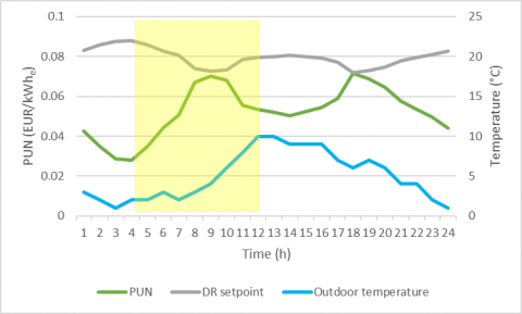
A typical trend for the PUN is represented in Figure 3, along with the outdoor air temperature and the indoor air setpoint temperature determined according to the DR strategy provided by the set of equations (2). In order to have an acceptable time for the experimentations, the time interval considered was not referred to an entire day, but only to 8 hours (from 04:00 AM to 12:00 AM, as highlighted in Figure 3).
Figure 3. PUN, indoor air setpoint temperature for the DR program and outdoor temperature
The delivery temperature of water in the condenser side of the heat pump was set in the range 50-55°C, to simulate a real application where fan coils are used as ambient terminals. The interaction between the DR program and the test rig implies that when the actual value of the indoor air temperature (Tair), determined with the thermal balance (1), is lower than the setpoint value (Tsp,i) determined with the algorithm (2), the electric pump in the circuit of cold water is activated and the fluid is allowed to absorb heat from the condenser side. This condition simulates the ON cycle of the heat pump, where the compressor is activated and there is absorption of electrical energy from the grid. During the ON cycle, the rotational speed of the electric pump is managed by the inverter, whose working frequency is controlled by means of a PID (proportional-integral-derivative) control defined in LabVIEW. On the other hand, when Tair > Tsp,i, the electric pump is deactivated, condition that simulates the OFF cycle of the heat pump.
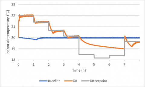
The evaluation of the effectiveness of the DR program was based on a comparison with a baseline, where the indoor air setpoint temperature was fixed at 20°C. Two tests with a duration of 8 hours were therefore carried out and their results will be discussed in this section. It should be noted that both the tests were started when the delivery temperature of water in the condenser side of the heat pump was 55°C and an initial condition of Tair = Tw = 20°C was imposed.
Figure 4 shows the trend of the indoor air temperature (Tair) for the baseline and the DR case. For the baseline condition, it can be seen that the actual indoor air temperature is kept nearly constant in a narrow range. As we will see later, this condition guarantees a high level of thermal comfort. For the DR program, instead, it is possible to note that the setpoint temperature is variable (with the PUN, according to the strategy (2)) and so it is the actual indoor air temperature. Based on the DR strategy, the indoor air temperature is higher when the PUN is lower than its average daily value, and lower when the PUN is higher than its average daily value. It is worth noting that in the time period when the PUN assumes its highest values, the actual indoor air temperature is about 1°C higher than that of the setpoint, because thermal energy was stored by the capacitance of the building during the first hours and then released. During this period, the compressor of the heat pump is not active, thus the absorption of electrical energy from the grid is limited to the auxiliary devices.
Figure 4. Indoor air temperature for the baseline and the DR program
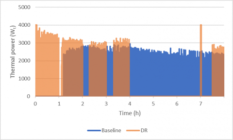
The thermal power released by the condenser of the heat pump to water is reported in Figure 5, for the baseline and the DR program. In the former case, there is basically a continuous heat transfer between the heat pump and the water, because to keep the indoor air temperature at its fixed setpoint value of 20°C, the compressor needs to be constantly active. In the latter case, instead, the release of thermal energy is not continuous, but only limited to the ON cycles when the compressor is required to be active. When the PUN assumes its highest values, there is no heat transfer between the heat pump and the water: the indoor air setpoint value is kept only thanks to the thermal capacitance of the building.
Figure 5. Thermal power output of the heat pump for the baseline and the DR program
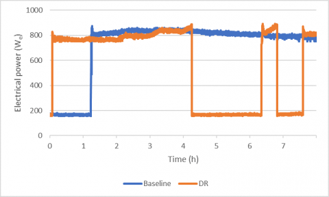
Figure 6 depicts the absorption of electrical energy from the heat pump, for the baseline and the DR case. As can be seen, when the compressor of the heat pump is not working, the absorption of the auxiliary devices is equal to about 160 We. Instead, during the ON cycles, the total absorption is between 800 and 900 We. For the baseline condition, the compressor is active for almost the entire duration of the test. For the DR condition, the compressor of the heat pump is on when the variable setpoint temperature of the indoor air is higher than 20°C. When the setpoint is lower than 20°C, the compressor is off; the second ON cycle that can be seen in Figure 6 is due to the fact that, in that period, the delivery temperature of water resulted to be lower than 50°C.
Figure 6. Electrical power absorbed by the heat pump for the baseline and the DR program
The overall electrical consumption and cost for the baseline and the DR program are provided in Table 2. It is worth noting that, for the baseline, a constant electricity price equal to the average value of the PUN was considered (0.052 EUR/kWhe). As indicated in Table 2, the percentage reduction that can be reached with the DR program for both the electrical consumption and its cost is relevant.
Table 2. Electrical consumption and cost for the baseline and the DR program
|
Case |
Electrical consumption (kWhe) |
Cost (EUR) |
|
BaselineTable size |
5.114 |
0.268 |
|
DR program |
4.187 |
0.199 |
|
Deviation |
-18.1% |
-25.7% |
Since with the DR program the indoor air temperature is allowed to vary in a wider range, it is important to check if the conditions of thermal comfort are respected. The predicted mean vote (PMV) of the virtual building was therefore determined using the model proposed by Buratti et al. [10]. This model correlates the PMV to the indoor air temperature and the partial pressure of the water vapor contained in the humid air (pv) as follows:
$P M V=a T_{\text {air }}+b p_{\mathrm{y}}-c$ (3)
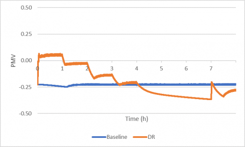
where, a, b and c are coefficients that depend on the gender of occupants and their clothing. Using the values that refer to both genders, clothes with a thermal resistance in the range 0.51-1 clo and imposing a design indoor relative humidity of 50%, the trend of the PMV for the present study can be visualized in Figure 7. As mentioned above, the PMV is nearly constant for the baseline condition, where the indoor air temperature varies in a narrow range. For the DR program, instead, the PMV is more variable and wider, however its values are always in the range between -0.5 and +0.5, condition that can be considered acceptable for the indoor thermal comfort.
Figure 7. PMV for the baseline and the DR program
In this work, the energy performance of a commercial air-to-water heat pump was experimentally evaluated when managed with a demand response (DR) program. The thermal load was associated to the space heating demand of a virtual building, which was modeled with a resistance-capacitance thermal network. The DR program, based on a real-time pricing control strategy, managed the interaction between the closed-loop system and the virtual building, which was able to unlock its energy flexibility thanks to a variable indoor air setpoint temperature. The results obtained with the DR program were compared with those of a baseline condition, obtained with a conventional control based on a fixed setpoint temperature.
The results of the study showed that the use of the DR program allowed to reduce electricity consumption and cost, without altering thermal comfort in a relevant way. Specifically, for the baseline condition the compressor of the heat pump resulted to be active for almost the entire duration of the test (85% of the time), with an absorption of 800-900 We. For the DR condition, instead, the compressor was on only when the strategy required a variable setpoint temperature of the indoor air higher than that of the baseline condition (20°C), or when the supply temperature of water was too low; this allowed to reduce the ON cycle of the compressor to 63% of the entire time of the test. Respect to the baseline, the DR program was able to reduce the overall absorption of electrical energy by -18.1%, and the total cost by -25.7%. While in the baseline the internal air temperature was constantly kept at 20°C, with the DR program the actual indoor air temperature was allowed to vary in the range 18-22°C. This variation led to a more variable predicted mean vote (PMV) for the DR case; however, it was verified that PMV was always in the range between -0.5 and +0.5, condition that can be considered acceptable for the indoor thermal comfort.
Based on the results of the study, it is possible to conclude that heat pumps, thanks to their thermal and demand-side flexibility potential, will play a key role in future energy systems and will be fundamental to achieve the 2050 climate targets defined by the EU.
|
a |
coefficient |
|
b |
coefficient |
|
C |
thermal capacitance, MJ/K |
|
c |
coefficient |
|
PMV |
predicted mean vote |
|
PUN |
Italian single price, EUR/kWhe |
|
p |
pressure, Pa |
|
Q |
thermal power, Wt |
|
R |
thermal resistance, K/W |
|
T |
temperature, °C |
|
t |
time, s |
|
Subscripts |
|
|
air |
indoor air |
|
amb |
ambient |
|
e |
external |
|
hp |
heat pump |
|
i |
internal |
|
i |
referred to the i-th hour |
|
max |
maximum |
|
min |
minimum |
|
sp |
setpoint |
|
tot |
total |
|
v |
vapor |
|
w |
wall |
|
Acronyms |
|
|
DIISM |
Department of Industrial Engineering and Mathematical Science |
|
DR |
Demand Response |
|
EPBD |
European Performance of Building Directive |
|
EU |
European Union |
|
HVAC |
Heating, Ventilation, and Air-Conditioning |
|
nZEB |
Nearly-Zero Energy Building |
|
PID |
Proportional-Integral-Derivative |
|
RES |
Renewable Energy Source |
|
TOU |
Time of Use |
[1] Jakubcionis, M., Carlsson, J. (2017). Estimation of European Union residential sector space cooling potential. Energy Policy, 101: 225-235. https://doi.org/10.1016/j.enpol.2016.11.047
[2] Santamouris, M., Kolokotsa, D. (2013). Passive cooling dissipation techniques for buildings and other structures: The state of the art. Energy and Buildings, 57: 74-94. https://doi.org/10.1016/j.enbuild.2012.11.002
[3] Poppi, S., Sommerfeldt, N., Bales, C., Madani, H., Lundqvist, P. (2018). Techno-economic review of solar heat pump systems for residential heating applications. Renewable and Sustainable Energy Reviews, 81: 22-32. https://doi.org/10.1016/j.rser.2017.07.041
[4] EU (European Union). Directive 2010/31/EU of the European Parliament and of the Council of 19 May 2010 on the Energy Performance of Buildings, 2010.
[5] EHPA. The European heat pump market has achieved double-digit growth for the fourth year in a row, 2019. https://www.ehpa.org/market-data/.
[6] Jensen, S.Ø., Marszal-Pomianowska, A., Lollini, R., Pasut, W., Knotzer, A., Engelmann, P., Reynders, G. (2017). IEA EBC annex 67 energy flexible buildings. Energy and Buildings, 155: 25-34. https://doi.org/10.1016/j.enbuild.2017.08.044
[7] Arteconi, A., Polonara, F. (2018). Assessing the demand side management potential and the energy flexibility of heat pumps in buildings. Energies, 11(7): 1846. https://doi.org/10.3390/en11071846
[8] Coccia, G., D’Agaro, P., Cortella, G., Polonara, F., Arteconi, A. (2019). Demand side management analysis of a supermarket integrated HVAC, refrigeration and water loop heat pump system. Applied Thermal Engineering, 152: 543-550. https://doi.org/10.1016/j.applthermaleng.2019.02.101
[9] Shen, B., Ghatikar, G., Lei, Z., Li, J., Wikler, G., Martin, P. (2014). The role of regulatory reforms, market changes, and technology development to make demand response a viable resource in meeting energy challenges. Applied Energy, 130: 814-823. https://doi.org/10.1016/j.apenergy.2013.12.069
[10] Buratti, C., Ricciardi, P., Vergoni, M. (2013). HVAC systems testing and check: A simplified model to predict thermal comfort conditions in moderate environments. Applied Energy, 104: 117-127. https://doi.org/10.1016/j.apenergy.2012.11.015