Antonio Rosato | Antonio Ciervo* | Renata Concetta Vigliotti | Roxana Adina Toma | Rossana Pellegrino | Giovanni Ciampi | Michelangelo Scorpio | Sergio Sibilio
OPEN ACCESS
In this paper 5 different case studies of solar hybrid heating and cooling networks serving 5 different school buildings assumed as representative of the 5 provinces of the Campania region (southern Italy) have been modelled, dynamically simulated and analyzed by means of the software TRNSYS over a 5-year period. The plants are based on the operation of solar thermal collectors coupled with a seasonal borehole thermal energy storage; the solar field is also integrated with photovoltaic panels coupled with an electric energy storage; a solar-powered adsorption system is used for covering the cooling requirements. Specific weather data files have been developed for each city based on 1-year in-situ hourly measurements to accurately take into account the influence of climatic conditions on systems’ performance; the effects of thermo-physical properties of underground associated to the different locations have also been taken into consideration according to measured data available in the literature. The proposed systems have been compared with conventional Italian heating and cooling plants from energy, environmental and economic points of view in order to assess the potential benefits, highlight the effects of both weather data and characteristics of underground as well as promote the diffusion of solar systems for Italian applications.
solar energy, borehole thermal energy storage, electric energy storage, adsorption chiller, weather data
Solar energy is abundant, free and non-polluting; therefore, it is considered one of the most competitive choices among all renewable sources able to ensure a sustainable future and address the increasingly serious impacts of climate change via either solar thermal collectors (SCs) and photovoltaic panels (PVs). Coupling battery storages (EB) with PVs could help in enhancing the self-consumption of electricity generated by PVs and, therefore, reducing the operating costs for end-users, limiting the stress on electric infrastructure during peak loads and improving power quality and reliability [1]; currently batteries represent mature energy storage devices with high energy densities and large potential applications [2]. However, solar energy is intermittent and a surplus is often available in summer months; this leads to a time discordance between solar supply and heat demand. Seasonal or long-term thermal energy storages allow for thermal energy storage over weeks and months, with it being a viable solution to overcome this temporal mismatch [3]. Numerous projects and installations have seen the light of day in Europe and North America, together with a number of scientific studies [4], highlighting promising performances of these systems. Even if four main types of seasonal storages have been presented by researchers, borehole thermal energy storage (BTES) is one of the most favorable according to Rad et al. [5]. A BTES consist of closed-loops where heat is charged or discharged by vertical or horizontal borehole heat exchangers (BHEs), which are installed into boreholes below the ground surface; after drilling, a U-pipe is inserted into the borehole and the borehole is then filled with a grouting material; the BHEs can be hydraulically connected in series or in parallel. The underground is used as storage material in a BTES, so that the performance of BTESs is strongly affected by the heat exchange capacity of the ground surrounding the BHEs, i.e. the stratigraphic succession and the hydrogeological conditions [6]. Solar energy could also be effectively used to activate adsorption chillers (ADHPs), mainly thanks to the fact that they could be driven at low supply temperatures (45÷65°C) [7, 8], avoiding the utilization of electrically-driven chillers. However, ADHPs are characterized by lower coefficients of performance (between 0.4 and 0.7) and higher unit cost for the same cooling capacity [7]; therefore, their utilization and potential benefits have to be investigated and assessed in more detail. Small ADHPs are recently being transferred into the market [7]. With reference to the Italian scenario, only five studies [9] analyzed the operation of solar heating systems integrating long-term thermal energy storages. However, they are very few and generally dated, with only two of these studies referring to the climatic conditions of southern Italy; in addition, the environmental and the economic impacts are neglected in most of these works; finally, these researches focus on districts much different from that one considered in this study. To the knowledge of the authors, there aren’t even any scientific paper focusing on performance of solar heating and cooling networks integrating both seasonal thermal energy storages and adsorption chillers (CSHCPSSs) operating in Italy [10]. Taking into account that climatic conditions could greatly affect the energy demand profiles of end-users, the design as well as the overall performance of CSHCPSSs, the literature review highlights that there is a specific need to perform additional investigations for Italian applications. In this paper, the performance of CSHCPSSs has been modelled, simulated and analyzed by means of the dynamic simulation TRNSYS [11] over a period of 5 years. The analysis has been performed by considering 5 different case studies consisting of school buildings located into 5 different cities belonging to the 5 different provinces of the Campania region (south of Italy). The climatic conditions as well as the properties of underground associated to each location have been accurately determined based on 1-year in-situ measurements as well as literature data. The performance of the CSHCPSSs have been assessed from energy, environmental and economic points of view and contrasted with the operation of typical Italian heating and cooling plants in order to estimate the potential benefits.
In this study 5 school buildings located into the 5 different cities (Avellino, Apollosa, Giano Vetusto, Acerra, Altavilla Silentina) belonging to the 5 different provinces (Avellino, Benevento, Caserta, Napoli, Salerno, respectively) of the Campania region (south of Italy) have been selected.
Table 1 highlights the geographic coordinates, the Heating Degree Days (HDD), the minimum/maximum outside temperature as well as the average global solar irradiation on a horizontal surface of the cities. The climatic data reported in this table have been derived based on 1-year in-situ hourly measurements obtained by means of specifically dedicated weather stations. This table shows that: a) the lowest minimum and the largest maximum annual outside temperature is achieved in Apollosa (-2.2°C and 38.2°C, respectively); b) the average annual global solar irradiation on a horizontal surface is maximum (352.3 Wh/m2) in Acerra and minimum (325.2 Wh/m2) in Giano Vetusto.
The cities where the school buildings are located are also characterized by different properties of underground. Table 2 indicates the number and depth of underground layers as well as the associated materials upon varying the location derived from the geographic data held by the Italian Institute for Environmental Protection and Research (ISPRA) [12]. The same table reports the main thermo-physical characteristics (thermal conductivity λ, specific heat cp and density ρ) of the underground materials according to the literature review [6]; these data represent “average” values taking into account that they depend on several factors such as temperature, porosity, water content, degree of saturation, pore fluid, dominant mineral phase, texture and mineralogical composition, etc. of materials [6].
Table 1. Minimum/maximum outside temperature and average global solar irradiation as a function of the city
|
|
Avellino |
Apollosa |
Giano Vetusto |
Acerra |
Altavilla Silentina |
|
Latitude |
40°55'13.39" North |
41°5'40.45" North |
41°12'10.02" North |
40°56'37.86" North |
40°31'56.27" North |
|
Longitude |
14°46'44.05" East |
14°42'16.35" East |
14°11'34.53" East |
14°22'57.51" East |
15°3'33.96" East |
|
HDD |
1742 |
1853 |
1497 |
1011 |
1536 |
|
|
Minimum/maximum outside temperature (°C) |
||||
|
Annual |
-0.8/35.4 |
-2.2/38.2 |
3.0/35.1 |
4.1/34.0 |
3.8/35.1 |
|
January |
-0.8/15.1 |
-2.2/17.8 |
4.5/17.5 |
6.9/15.8 |
7.6/15.6 |
|
February |
-0.7/15.7 |
-1.2/18.8 |
4.3/17.3 |
6.4/17.4 |
5.5/17.9 |
|
March |
0.5/20.9 |
-2.1/22.8 |
3./22.0 |
4.1/18.9 |
3.8/17.4 |
|
April |
-0.2/25.5 |
-1.5/27.7 |
3.4/24.5 |
5.3/20.6 |
4.4/20.5 |
|
May |
7.5/30.1 |
6.0/31.2 |
13.5/30.2 |
14.1/33.3 |
13.3/35.1 |
|
June |
9.7/33.2 |
9.8/34.2 |
15.1/33.5 |
16.6/31 |
14.9/30.1 |
|
July |
15.5/35.4 |
15.4/38.2 |
20.2/35.1 |
21.7/32.3 |
20.8/31.8 |
|
August |
16.6/34.5 |
17.4/36.7 |
18.6/34.9 |
19.5/34 |
19/33.4 |
|
September |
9.1/32.3 |
10.3/35.3 |
13.3/34.6 |
13.8/32.5 |
14.8/33.1 |
|
October |
6.2/28.0 |
6.7/31.2 |
11.2/29.6 |
13.2/25.6 |
13/28 |
|
November |
3.1/20.3 |
4.6/23.5 |
8.4/23.2 |
8.6/22.7 |
9.9/21.3 |
|
December |
0.9/17.2 |
0.1/18.3 |
6.7/18.7 |
7.8/18.5 |
7.7/20.2 |
|
|
Average global solar irradiation on a horizontal surface (W/m2) |
||||
|
Annual |
340.6 |
345.9 |
325.2 |
352.3 |
345.5 |
|
January |
219.2 |
218.2 |
197.2 |
221.5 |
228.1 |
|
February |
258.7 |
283.3 |
235.3 |
274.4 |
262.5 |
|
March |
334.7 |
320.7 |
295.0 |
322.2 |
342.5 |
|
April |
404.8 |
424.7 |
395.2 |
407.4 |
404.7 |
|
May |
407.1 |
397.1 |
378.6 |
397.5 |
407.7 |
|
June |
420.9 |
421.6 |
414.7 |
472.1 |
430.3 |
|
July |
462.0 |
460.4 |
468.0 |
483.3 |
467.0 |
|
August |
426.4 |
436.9 |
403.6 |
447.2 |
432.1 |
|
September |
348.7 |
361.6 |
336.2 |
367.3 |
350.1 |
|
October |
272.9 |
282.8 |
252.6 |
275.3 |
277.0 |
|
November |
196.1 |
191.9 |
193.6 |
210.3 |
206.0 |
|
December |
144.4 |
141.6 |
144.3 |
152.1 |
148.8 |
Table 2. Properties of underground layers [6]
|
Location |
Layer depth (m) |
Material |
λ (W/mK) |
cp (kJ/kgK) |
ρ (103kg/m3) |
|
Avellino |
0÷10 |
Soil |
2.50 |
0.87 |
2.65 |
|
10÷50 |
Clay-mudstone |
2.04 |
0.91 |
2.50 |
|
|
50÷80 |
Limestone |
2.81 |
0.89 |
2.55 |
|
|
Apollosa |
0÷6 |
Marlstone |
2.34 |
0.93 |
2.45 |
|
6÷15 |
Tuff |
0.41 |
0.89 |
1.30 |
|
|
15÷30 |
Clean gravel, dry |
0.52 |
0.74 |
2.00 |
|
|
Giano Vetusto |
0÷1.5 |
Soil |
2.50 |
0.87 |
2.65 |
|
1.5÷8 |
Silt and clay, dry |
0.79 |
0.82 |
1.90 |
|
|
8÷52 |
Medium sand, dry |
0.53 |
0.74 |
2.00 |
|
|
52÷80 |
Clay-mudstone |
2.04 |
0.91 |
2.50 |
|
|
Acerra |
0÷3 |
Soil |
2.50 |
0.87 |
2.65 |
|
3÷12 |
Tuff |
0.41 |
0.89 |
1.30 |
|
|
12÷24 |
Medium sand, dry |
0.53 |
0.74 |
2.00 |
|
|
24÷60 |
Tuff |
0.41 |
0.89 |
1.30 |
|
|
Altavilla Salentina |
0÷4 |
Soil |
2.50 |
0.87 |
2.65 |
|
4÷12 |
Clay, dry |
0.89 |
0.82 |
1.90 |
|
|
12÷16 |
Silt and clay, dry |
0.79 |
0.82 |
1.90 |
|
|
16÷22 |
Clean gravel, dry |
0.52 |
0.74 |
2.00 |
|
|
22÷40 |
Sandstone |
3.61 |
0.93 |
2.45 |
|
|
40÷46 |
Marlstone |
2.34 |
0.93 |
2.45 |
|
|
46÷54 |
Sandstone |
3.61 |
0.93 |
2.45 |
Table 3. Description of school buildings
|
|
Avellino |
Apollosa |
Giano Vetusto |
Acerra |
Altavilla Silentina |
|
Year of construction |
1976 |
1973 |
1961 -1975 |
After 1976 |
1950 |
|
Number of floors |
2 |
3 |
1 |
2 |
1 |
|
Total floor area (m2) |
1656.2 |
1686.6 |
675.4 |
5246.2 |
265.7 |
|
Windows’ area (m2) |
132.3 |
172.8 |
33.6 |
366.1 |
21.4 |
|
Volume (m3) |
5542.5 |
6913.8 |
2377.4 |
15763.7 |
818.2 |
|
Maximum number of simultaneous occupants |
212 |
243 |
47 |
637 |
53 |
In addition to the climatic conditions and properties of underground, the selected school buildings differ in terms of number of floors, floor area, windows’ area, volume as well as maximum simultaneous occupants, as indicated in Table 3. Thermal transmittance of windows has been calculated by means of the Standard UNI EN ISO 10077-1 according to the geometry and materials of frames and glazings; thermal transmittance of opaque elements of buildings’ envelope has been calculated by means of the Standard UNI EN ISO 6946 according to the material and thickness of layers composing walls, floors and ceilings.
The air change of infiltration has been assumed equal to 0.24 h–1 during the heating period (whatever the outside temperature is); during the summer, it has been assumed equal to 0.24 h–1 when the outdoor temperature is greater than 26°C and equal to 0.6 h–1 when the ambient temperature is lower than 26°C in order to take into account the more frequent openings of windows (according to Zarrella et al. [13]). The occupancy profiles of schools have been defined according to the official schools’ timetable for a period ranging between September 15th and June 30th (except weekends and periods of school holidays). The annual electric demand profiles have been derived according to the occupancy profiles by considering the operation of lighting systems as well as PCs. The annual internal gain profiles have been set based on the occupancy profiles by assuming a heat gain of 75 W/occupant together with 140 W for each PC; a heat gain equal to 70% of nominal electric power has been considered for lighting systems. The domestic hot water demand has been neglected for the school buildings.
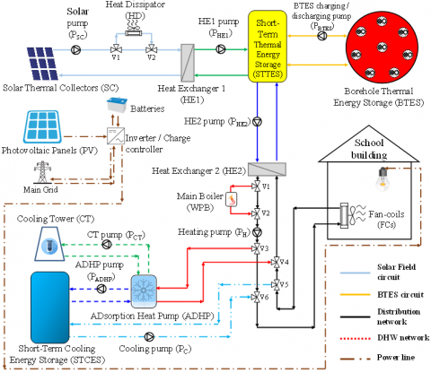
Figure 1 shows the scheme of the proposed Central Solar Heating and Cooling Plant with Seasonal Storage (CSHCPSS).
Figure 1. Schematic of the proposed CSHCPSS
A water-ethylene glycol mixture (60%/40% by volume) is used as heat carrier fluid. The solar energy captured by the solar thermal collectors (SCs) installed on the roofs is firstly transferred, through the heat exchanger HE1, into the vertical cylindrical short-term thermal energy storage (STTES); solar thermal energy surplus is dissipated by blowing air across a finned coil heat dissipator (HD) when the outlet temperature of SCs is higher than 95°C and, therefore, prevent the boiling of the heat carrier fluid. During the cooling period, solar energy is moved from the STTES to the adsorption chiller (ADHP) by means of the heat exchanger HE2; this allows obtaining the desired cooling energy to be stored into the vertical cylindrical short-term cooling energy storage (STCES) and then provided to the schools for cooling purposes. During the heating period, solar energy stored into the STTES can be moved, through the HE2, into the distribution network and, then, into the fan coils installed inside the buildings to cover the heating load. If the solar energy is not immediately required for space heating/cooling purposes, it can be moved from the STTES to the BTES (with vertical single U-pipes borehole heat exchangers) during the whole year (“BTES charging mode”). Only during the heating season, thermal energy stored in the BTES field can return into the STTES (“BTES discharging mode”) to integrate the temperature level. A centralized boiler (WPB), fueled with pellets, is eventually used as back-up unit with the aim of integrating the solar contribution and maintaining the desired supply temperature. The electricity delivered by the PVs is primarily utilized to satisfy the electric demand of end-users and plant components, while the excess is transferred into the batteries (EB) only when their charging status is lower than 100%; the batteries are discharged only when their charging status is larger than 10%. In the case of the electric energy generated by the PVs is greater than the overall electric load and the batteries charging level is equal to 100%, the electric production that cannot be charged into the batteries is then sold to the central grid. The central grid, as well as the batteries, are utilized to satisfy the peaks of electric load. Table 4 details the most important characteristics of the main CSHCPSS components as a function of the location.
Table 4. Characteristics of the main components of the CSHCPSS
|
|
Avellino |
Apollosa |
Giano Vetusto |
Acerra |
Altavilla Silentina |
|
SCs [14] |
|||||
|
Type / model |
Flat plate / FSK 2.5 |
||||
|
Total aperture area (m2) |
103.95 |
124.74 |
41.58 |
464.31 |
34.65 |
|
Orientation / tilted angle / azimuth |
South / 30° / 0° |
||||
|
PVs [15] |
|||||
|
Type / model |
Monocrystalline / BP SOLAR |
||||
|
Total area (m2) |
282.24 |
120.96 |
866.88 |
40.32 |
|
|
Orientation / tilted angle / azimuth |
South / 30° / 0° |
||||
|
STTES [16] |
|||||
|
Volume (m3) |
9.8 |
11.8 |
4.0 |
45.6 |
3.3 |
|
STCES [16] |
|||||
|
Volume (m3) |
3.9 |
4.7 |
0.9 |
18.2 |
1.3 |
|
Battery [17] |
|||||
|
Single battery usable capacity (kWh) |
13.5 |
||||
|
Number of series-connected batteries |
8 |
4 |
32 |
2 |
|
|
BTES |
|||||
|
Volume (m3) |
272.8 |
276.1 |
325.3 |
921.7 |
54.1 |
|
Number of series-connected boreholes |
8 |
1 |
|||
|
Borehole depth (m) |
7.78 |
7.88 |
9.28 |
26.30 |
12.35 |
|
λ of underground (W/mK) |
2.50 |
1.62 |
1.00 |
0.66 |
0.56 |
|
U-pipe spacing (m) |
0.05 |
||||
|
WPB [18] |
|||||
|
Model |
GEYSIR 46,5 |
GEYSIR 34 |
GEYSIR 46,5 |
GEYSIR 34 |
|
|
Rated capacity of a single boiler (kW) |
46.5 |
31.8 |
46.5 |
31.8 |
|
|
Number of series-connected boilers |
3 |
1 |
6 |
1 |
|
|
ADHP [19] |
|||||
|
Model |
eCoo 40X |
eCoo 20ST |
eCoo 30 |
eCoo 20ST |
|
|
Number of parallel-connected units |
1 |
5 |
1 |
||
|
Cooling capacity of unit (kW) |
100.0 |
100.0 |
33.4 |
50.0 |
33.4 |
The total aperture area of solar thermal collectors, the volume of the STTES, the volume of the STCES as well as the volume of the BTES have been determined based on energy demands of the buildings and according to the results of a huge sensitivity analysis performed by the authors in a previous study [10]. Thermal conductivity of underground is an ‘equivalent’ value representative for the entire stratigraphic sequence; it has been obtained as the weighted average of the entire depth of the BHEs calculated by taking into account the thickness of each lithology. A specifically dedicated material [20] has been used for grouting the boreholes. The area of PVs for each building has been selected in order to cover the related maximum power demand, while the total capacity of batteries has been defined based on the daily average overall electricity consumption of schools. The sizes of both WPB and ADHPs have been set according to the thermal/cooling load profiles of each school in order to guarantee the desired thermal comfort at least 90% of the time.
A conventional decentralized heating and cooling system (CS) has been assumed as reference system and, therefore, modeled and simulated for each school building to be compared with the proposed CSHCPSS while serving the same end-users. According to the current Italian scenario, a natural gas-fired boiler (NGB) coupled with radiators is considered for space heating purposes, while the cooling demand is covered by means of a typical multi-split air-to-air vapor compression electric refrigeration unit (RU). The size of components has been determined according to the energy demands of schools.
Both proposed and reference heating and cooling systems have been modeled, simulated and analyzed by means of the TRaNsient SYStems (TRNSYS) software platform 17. This tool uses a component-based methodology in which (i) a system is decomposed into components’ mathematical models (named “Types”), each of which is described by a FORTRAN subroutine, (ii) the user assembles the Types by linking component inputs and outputs and by assigning component performance parameters, and (iii) the program solves the resulting non-linear algebraic and differential equations to determine system response at each time step. In this study, detailed simulation models have been applied to each component which fully account for (i) transient nature of building and occupant driven loads, (ii) part-load characteristics of components, (iii) interaction between the loads and the system output, and (iv) system energy management and control. In this paper, the Types have been selected from the TRNSYS libraries and enhanced by experimental measurements and/or manufactures performance data and/or information available in current scientific literature according to the common characteristics of the components used in practice. The duration of simulation period (5 years) has been defined in order to consider that it takes time to fully charge the seasonal storage. A simulation time step of 1 minute has been used, while January 1st has been assumed as starting date of the simulations. The Type 56 has been used to accurately model the envelopes of buildings (windows, walls, roofs and floors) as well as the occupant driven loads. The Type 557a [21], adopted to model the BTES, is considered to be the state-of-the-art in dynamic simulation of ground heat exchanger that interacts thermally with the ground. The storage volume has the shape of cylinder with vertical symmetry axis. The layout of the borehole field is fixed hexagonally and uniformly within the storage volume in the simulation. The STTES and STCES have been modelled by means of the Type 534 with 10 isothermal temperature layers to better represent the stratification in the tank, where the top layer is 1 and the bottom layer is 10; the tank model has been calibrated based on manufacturer data [16]. The flat-plate solar thermal collectors have been modelled by using the Type 1b, where the collector efficiency has been modelled by a second-order equation and correction for off-normal solar incidence is applied by a second-order incidence angle modifier according to the manufacturer data [14]. The model of PVs is described in De Soto et al. [15]; it is a five-parameter model able to predict the power delivered to the load. The battery is modelled with the Type 47a, while the inverter/charge controller is modelled with the Type 48b. The Type 47a specifies how the battery state of charge varies over time, given the rate of charge or discharge (it has been calibrated based on manufacturer data [17]); the Type 48b is composed of two devices, where the first one is a regulator which distributes DC power from the solar cell array to and from a battery (in systems with energy storage), while the second component is the inverter. The Type 700 has been used for modeling the WPB; according to the manufacturer performance data [18], its efficiency has been evaluated as a function of the thermal power output. The Type 31 has been used to model the pipes and calculate the related heat losses by assuming a loss coefficient equal to 0.05 kJ/(hm2K). The heating/cooling pumps have been modelled by the Type 742, while the other pumps in the system have been modelled by means of the Type 656. The Type 909 is used for the ADHP; this component models an adsorption chiller, relying on user-provided performance data files containing normalized capacity and COP ratios as a function of the hot water inlet temperature, the cooling water inlet temperature and the chilled water inlet temperature (suggested by the manufacturer [19]). Five specific weather data files have been created for each location based on 1-year in-situ measurements of key-parameters (outside air temperature, relative humidity, wind velocity and global solar irradiation on a horizontal surface) every hour in order to model the climatic conditions; the weather data are one year long and, therefore, have to be the same each year. With reference to the CS, the Type 700 has been used for modelling the natural gas-fired boiler (assumed with a constant thermal efficiency of 90.0%), while the radiators have been simulated by means of the Type 1231. The Type 941 has been adopted to model the performance of the refrigeration unit; this Type is able to provide the cooling/heating outputs, the power absorbed as well as the temperature of both heat carrier fluid and air according to the performance map suggested by the manufacturer [22]. Table 5 reports the TRNSYS control strategies for the activation/deactivation of the main components of both CSHCPSS and reference systems, whatever the location is. The heating season ranges from November 15st up to March 31st for Acerra, while for the other cities it covers the period November 1st-April 15th); the cooling season relates to the remaining part of the year. The target of indoor air temperature Troom is set to 20.0°C and 26.0°C (with a deadband of 0.5°C), respectively, during the heating and cooling seasons only in the case of at least one occupant being inside the buildings.
Table 5. Control strategies of main components of plants
|
|
OFF |
ON |
|
|
CSHCPSS |
|
|
Fan-coils (FCs) |
Heating season: Troom≥20.5°C Cooling season: Troom≤25.5°C |
Heating season: Troom≤19.5°C Cooling season: Troom≥26.5°C |
|
Solar pump & HE1 pump |
(TSC,out - T10,STTES)≤2°C OR T1,STTES > 90°C |
(TSC,out - T10,STTES)≥10°C AND T1,STTES≤90°C |
|
BTES charging / discharging pump |
Charging mode Heating season: (T10,STTES – 20°C)≤2°C OR T1,STTES≤55°C OR (T1,STTES - TBTES,center)≤2°C Cooling season: (T1,STTES - TBTES,center)≤2°C disCharging mode Heating season: (TBTES,center - T10,STTES)≤2°C OR T1,STTES > 65°C OR Solar pump ON |
Charging mode Heating season: (T10,STTES – 20°C) ≥10°C AND T1,STTES≥60°C AND (T1,STTES - TBTES,center)≥10°C Cooling season: (T1,STTES - TBTES,center)≥10°C disCharging mode Heating season: (TBTES,center - T10,STTES)≥5°C AND T1,STTES≤60°C AND Solar pump OFF |
|
ADHP pump and CT pump |
Heating season OR (Cooling season AND T6,STCES≤10°C) |
Cooling season AND T6,STCES≥13°C |
|
Heating pump |
Heating season: Troom≥20.5°C Cooling season: T6,STCES≤10°C |
Heating season: Troom≤19.5°C Cooling season: T6,STCES≥13°C |
|
Cooling pump |
Heating season OR (Cooling season AND Troom≤25.5°C) |
Cooling season AND Troom≥26.5°C |
|
HE2 pump |
Heating pump OFF OR (Tin,HE2,hot – Tin,HE2,cold)≤2°C |
Heating pump ON AND (Tin,HE2,hot – Tin,HE2,cold )≥5°C) |
|
WPB |
Heating season: Tout,WPB≥55°C Cooling season: ADHP pump OFF OR Tout,WPB≥75°C |
Heating season: Tin,WPB < 50°C Cooling season: ADHP pump ON AND Tin,WPB < 70°C |
|
|
CS |
|
|
Boiler |
Heating season: Troom≥20.5°C |
Heating season: Troom≤19.5°C |
|
RU |
Cooling season: Troom≤25.5°C |
Cooling season: Troom≥26.5°C |
The simulation results obtained as outputs of the TRNSYS Types associated to the operation of every single component of the CSHCPSSs have been analyzed and compared with those associated to the CSs, assumed as reference, from energy, environmental and economic points of view as described below.
The energy comparison between the proposed and conventional systems has been performed in terms of primary energy consumption by means of the index named Primary Energy Saving (PES):
$\mathrm{PES}=\left(\mathrm{E}_{\mathrm{p}}^{\mathrm{CS}}-\mathrm{E}_{\mathrm{p}}^{\mathrm{CSHCPSS}}\right) / \mathrm{E}_{\mathrm{p}}^{\mathrm{CS}}$ (1)
where, EpCSHCPSS is the primary energy consumed by the CSHCPSSs and EpCS is the primary energy consumption of the CSs. The values of EpCSHCPSS and EpCS are calculated as follows:
$\mathrm{E}_{\mathrm{p}}^{\mathrm{CSHCPSS}}=\mathrm{E}_{\text {el,import }}^{\mathrm{CSHCPSS}} / \eta_{\mathrm{PP}}$ (2)
$\mathrm{E}_{\mathrm{p}}^{\mathrm{CS}}=\mathrm{E}_{\mathrm{th}, \mathrm{NGB}}^{\mathrm{CS}} / \eta_{\mathrm{NGB}}^{\mathrm{CS}}+\mathrm{E}_{\mathrm{el}, \text { import }}^{\mathrm{CS}} / \eta_{\mathrm{PP}}$ (3)
where: $\mathrm{E}_{\text {el,import }}^{\text {CSHCPSS }}$ and $\mathrm{E}_{\text {el,import }}^{\mathrm{CS}}$ are, respectively, the electricity imported from the central electric grid by the CSHCPSSs and the CSs; ηPP is the power plant average efficiency including transmission losses, in Italy (assumed equal to 0.42 [10]); $\text{ }\!\!\eta\!\!\text{ }_{\text{NGB}}^{\text{CS}}$ and $\mathrm{E}_{\mathrm{th}, \mathrm{NGB}}^{\mathrm{CS}}$ are, respectively, the thermal efficiency of NGB and energy provided by NGB.
The assessment of environmental impact has been performed in this study through an energy output-based emission factor approach [23] in terms of global carbon dioxide equivalent emissions by means of the parameter ∆CO2:
$\Delta \mathrm{CO}_{2}=\left(\mathrm{m}_{\mathrm{CO}_{2}}^{\mathrm{CS}}-\mathrm{m}_{\mathrm{CO}_{2}}^{\mathrm{CSHCPSS}}\right) / \mathrm{m}_{\mathrm{CO}_{2}}^{\mathrm{CS}}$ (4)
where, $\mathrm{m}_{\mathrm{CO}_{2}}^{\text {CSHPSS }}$ is the mass of the CO2 equivalent emissions associated to the CSHCPSSs and $\mathrm{m}_{\mathrm{CO}_{2}}^{\mathrm{CS}}$ is the mass of the CO2 equivalent emissions associated to the CSs. The values of $\mathrm{m}_{\mathrm{CO}_{2}}^{\mathrm{CSHCPSS}}$ and $\mathrm{m}_{\mathrm{CO}_{2}}^{\mathrm{CS}}$ used in Eq. (4) have been computed as reported below according to the method suggested by Chicco and Mancarella [23]:
$\mathrm{m}_{\mathrm{CO}_{2}}^{\mathrm{CSHCPSS}}=\beta_{\mathrm{WP}} \cdot \mathrm{E}_{\mathrm{th}, \mathrm{WPB}}^{\mathrm{CSHCPSS}} / \eta_{\mathrm{WPB}}^{\mathrm{CSHCPSS}}+\alpha \cdot \mathrm{E}_{\mathrm{el}, \text { import }}^{\mathrm{CSHCPSS}}$ (5)
$\mathrm{m}_{\mathrm{CO}_{2}}^{\mathrm{CS}}=\beta_{\mathrm{NG}} \cdot \mathrm{E}_{\mathrm{th}, \mathrm{NGB}}^{\mathrm{CS}} / \eta_{\mathrm{NGB}}^{\mathrm{CS}}+\alpha \cdot \mathrm{E}_{\mathrm{el}, \mathrm{import}}^{\mathrm{CS}}$ (6)
where, βWP is the CO2 equivalent emission factor associated to the wood pellet consumption [24]; α is the CO2 equivalent emission factor for electricity production [10]; βNG represents the CO2 equivalent emission factor associated to the primary energy associated to natural gas consumption [10]. According to the values suggested in [10] with reference to the Italian scenario, in this study α, βNG and βWP have been assumed equal to 573.0 gCO2/kWhel, 207.0 gCO2/kWhp and 49.0 gCO2/kWhp, respectively.
The economic analysis has been performed by comparing the operating costs of the proposed systems $\mathrm{OC}^{\mathrm{CSHCPSS}}$ with those of the reference systems $\mathrm{OC}^{\mathrm{CS}}$ as follows:
$\Delta \mathrm{OC}=\left(\mathrm{OC}^{\mathrm{CS}}-\mathrm{OC}^{\mathrm{CSHCPSS}}\right) / \mathrm{OC}^{\mathrm{CS}}$ (7)
The values of OCCS and OCCSHCPSS used in Eq. (7) have been computed as reported below:
$\mathrm{OC}^{\mathrm{CSHCPSS}}=\mathrm{UC}_{\mathrm{WP}} \cdot \mathrm{E}_{\mathrm{th}, \mathrm{WPB}}^{\mathrm{CSHCPSS}} /\left(\mathrm{LHV}_{\mathrm{WP}} \cdot \eta_{\mathrm{WPB}}^{\mathrm{CSHCPSS}}\right)$
$+\mathrm{UC}_{\mathrm{el}, \text { import }} \cdot \mathrm{E}_{\mathrm{el}, \mathrm{import}}^{\mathrm{CSHCPSS}}-\mathrm{UC}_{\mathrm{el}, \text { exported }} \cdot \mathrm{E}_{\mathrm{el} \text {,exported }}^{\mathrm{CSHCPSS}}$ (8)
$\mathrm{OC}^{\mathrm{CS}}=\mathrm{UC}_{\mathrm{NG}} \cdot \mathrm{E}_{\mathrm{th}, \mathrm{NGB}}^{\mathrm{CS}} /\left(\mathrm{LHV}_{\mathrm{NG}} \cdot \rho_{\mathrm{NG}} \cdot \eta_{\mathrm{NGB}}^{\mathrm{CS}}\right)$
$+\mathrm{UC}_{\mathrm{el} \text { limport }} \cdot \mathrm{E}_{\mathrm{el}, \text { import }}^{\mathrm{CS}}$ (9)
where, UCWP is the unit cost of wood pellet (assumed equal to 0.290 €/kg [24]), LHVWP is the lower heating value of wood pellet (assumed equal to 16,704.30 kJ/kg according to [25]), UCel,import is the unit cost of electric energy purchased from the central grid [26], UCel,sold is the unit revenue of the electricity sold to the central grid [27], UCNG is the unit cost of natural gas [26], LHVNG is the lower heating value of natural gas (assumed equal to 49,599 kJ/kg [10]), ρNG is the density of natural gas (assumed equal to 0.72 kg/m3 [10]). The tariffs of both electric energy as well as natural gas have been kept up-to-date according to the Italian scenario [24, 26, 27].
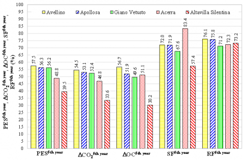
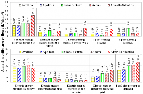
Table 6 reports the annual primary energy consumption, the annual mass of equivalent CO2 emissions and the annual operating costs of the CS assumed as baseline upon varying the location. The simulation results highlighted that the values of PES (Eq. (1)), $\Delta$CO2 (Eq. 4) and $\Delta$OC (Eq. (7)) are substantially constant upon varying the year of simulation, whatever the city is. Figure 2 indicates the values of PES5th year, $\Delta$CO25th year and $\Delta$OC5th year, solar fraction SF (defined as the percentage of the total thermal energy demand for heating/cooling purposes covered by solar energy) as well as the total renewable energy fraction RF (defined as the percentage of the total energy demand covered by renewable sources) associated to the 5th year of operation as a function of the city. Figure 3 highlights the main annual energy flows associated to the 5th year of simulation of the CSHCPSS divided by the floor area (indicated in Table 3) upon varying the city; in particular, the net solar energy recovered from SCs, the thermal energy injected into the BTES, the thermal energy supplied by the WPB, the space heating/cooling demands, the electric energy generated by PVs, the electric energy exported into the grid, the electric energy charged into the batteries and the electric energy imported from the grid and the total electric demand are indicated in this figure.
Figures 2-3 show that:
Table 6. Annual performance of the CSs
|
|
Avellino |
Apollosa |
Giano Vetusto |
Acerra |
Altavilla Silentina |
|
Primary energy consumption (MWh) |
93.3 |
104.5 |
58.5 |
401.9 |
23.4 |
|
Mass of equivalent CO2 emissions (MgCO2) |
22.0 |
24.7 |
13.6 |
95.5 |
5.5 |
|
Operating cost (k€) |
11.7 |
12.4 |
7.2 |
52.9 |
3.1 |
Figure 2. PES, $\Delta$CO2, $\Delta$OC, SF and RF associated to the 5th year of simulation as a function of the city
Figure 3. Main annual specific energy flows during the 5th year of simulation upon varying the city
The performance of solar hybrid heating and cooling networks integrated with borehole thermal energy storages have been simulated and assessed while serving typical school buildings of southern Italy and compared with those of conventional plants upon varying both weather conditions and underground properties. The simulations highlighted that the proposed systems are able to reduce the primary energy consumption, the equivalent CO2 emissions and the operating costs up to 57.5%, 54.5% and 56.7%, respectively.
This study has been undertaken within the research project entitled “Solar smart Energy Networks integrated with borehole thermal Energy storages serving small-scale districts in the CAmpania region - S.E.N.E.CA.” funded by the “V:ALERE 2019 program” of the University of Campania Luigi Vanvitelli (Italy).
|
cp |
specific heat, kJ. kg-1. K-1 |
|
E |
energy, MWh/kWh |
|
LHV |
lower heating value, kJ. kg-1 |
|
m |
mass, kg/Mg |
|
OC |
operating cost, €/k€ |
|
PES |
primary energy saving,% |
|
RF |
renewable fraction,% |
|
T |
temperature,°C |
|
UC |
unit cost, €. kWh-1/€. m-3 |
|
Greek symbols |
|
|
α |
CO2 emission factor for electricity production, gCO2. kWhel-1 |
|
β |
CO2 emission factor of natural gas consumption, gCO2. kWhp-1 |
|
∆ |
difference,% |
|
η |
efficiency,% |
|
λ |
thermal conductivity, W. mK-1 |
|
ρ |
density, kg. m-3 |
|
Subscripts and superscripts |
|
|
1 |
node 1 of the STTES |
|
6 |
node 6 of the STCES |
|
10 |
node 10 of the STTES |
|
5th year |
referred to the fifth year of simulation |
|
BTES |
borehole thermal energy storage |
|
center |
center of BTES |
|
CO2 |
carbon dioxide equivalent emissions |
|
cold |
load side |
|
CS |
conventional system |
|
CSHCPSS |
central solar heating and cooling plant with seasonal storage |
|
el |
electric |
|
exported |
exported to the grid |
|
HE2 |
heat exchanger 2 |
|
import |
imported from the grid |
|
hot |
source side |
|
in |
inlet |
|
NG |
natural gas |
|
NGB |
natural-gas fired boiler |
|
out |
outlet |
|
p |
primary |
|
PP |
power plant |
|
room |
indoor air |
|
SC |
solar collector |
|
STCES |
short-term cooling energy storage |
|
STTES |
short-term thermal energy storage |
|
th |
thermal |
|
WP |
wood pellet |
|
WPB |
wood pellet boiler |
[1] O'Shaughnessy, E., Cutler, D., Ardani, K., Margolis, R. (2018). Solar plus: Optimization of distributed solar PV through battery storage and dispatchable load in residential buildings. Applied Energy, 213: 11-21. https://doi.org/10.1016/j.apenergy.2017.12.118
[2] Koohi-Fayegh, S., Rosen, M.A. (2020). A review of energy storage types, applications and recent developments. Journal of Energy Storage, 27: 101047. https://doi.org/10.1016/j.est.2019.101047
[3] Hesaraki, A., Holmberg, S., Haghighat, F. (2015). Seasonal thermal energy storage with heat pumps and low temperatures in building projects-A comparative review. Renewable and Sustainable Energy Reviews, 43: 1199-1213. https://doi.org/10.1016/j.rser.2014.12.002
[4] IEA-SHC. IEA-SHC - Task 32 - Advanced storage concepts for solar and low energy buildings. Available: http://task32.iea-shc.org/
[5] Rad, F.M., Fung, A.S., Rosen, M.A. (2017). An integrated model for designing a solar community heating system with borehole thermal storage. Energy for Sustainable Development, 36: 6-15. https://doi.org/10.1016/j.esd.2016.10.003
[6] Dalla Santa, G., Galgaro, A., Sassi, R., Cultrera, M., Scotton, P., Mueller, J., ..., Bernardi, A. (2020). An updated ground thermal properties database for GSHP applications. Geothermics, 85: 101758. https://doi.org/10.1016/j.geothermics.2019.101758
[7] Hassan, A.A., Elwardany, A.E., Ookawara, S., Ahmed, M., El-Sharkawy, I.I. (2020). Integrated adsorption-based multigeneration systems: A critical review and future trends. International Journal of Refrigeration, 116: 129-145. https://doi.org/10.1016/j.ijrefrig.2020.04.001
[8] Rosato, A., Sibilio, S. (2013). Preliminary experimental characterization of a three-phase absorption heat pump. International Journal of Refrigeration, 36(3): 717-729. https://doi.org/10.1016/j.ijrefrig.2012.11.015
[9] Rosato, A., Ciervo, A., Ciampi, G., Scorpio, M., Guarino, F., Sibilio, S. (2020). Impact of solar field design and back-up technology on dynamic performance of a solar hybrid heating network integrated with a seasonal borehole thermal energy storage serving a small-scale residential district including plug-in electric vehicles. Renewable Energy, 154: 684-703. https://doi.org/10.1016/j.renene.2020.03.053
[10] Rosato, A., Ciervo, A., Guarino, F., Ciampi, G., Scorpio, M., Sibilio, S. (2020). Dynamic simulation of a solar heating and cooling system including a seasonal storage serving a small Italian residential district. Thermal Science, 24: 3555-3568. https://doi.org/10.2298/TSCI200323276R.
[11] TRNSYS. The transient energy system simulation tool. Available: http://www.trnsys.com
[12] ISPRA. Geological Survey of Italy Portal. Available: http://sgi2.isprambiente.it/
[13] Zarrella, A., De Carli, M., Peretti, C. (2014). Radiant floor cooling coupled with dehumidification systems in residential buildings: A simulation-based analysis. Energy Conversion and Management, 85: 254-263. https://doi.org/10.1016/j.enconman.2014.05.097
[14] Kloben. FSK model. Available: http://www.kloben.it/products/view/3.
[15] De Soto, W., Klein, S.A., Beckman, W.A. (2006). Improvement and validation of a model for photovoltaic array performance. Solar Energy, 80(1): 78-88. https://doi.org/10.1016/j.solener.2005.06.010
[16] Paradigma. PS series. Available: http://www.paradigmaitalia.it/serbatoio-accumulo-acqua-calda-riscaldamento/boiler-accumulo-acqua-calda/accumulo-solare-termico
[17] TESLA. Powerwall Battery. Available: https://www.tesla.com/powerwall?redirect=no
[18] FAMAR. GEYSIR. Available: https://famarbrevetti.com/caldaia-pellet-policombustibile/#1500734921869-71635334-cf2d
[19] FAHRENHEIT GmbH. eCoo30. Available: https://fahrenheit.cool/en/products/chillers/ecoo/
[20] CETCO. GEOTHERMAL GROUT. Available: http://www.continentaldrillingsupply.com/GEOTHERMAL-GROUT.pdf
[21] Hellström, G. (1989). Heat Storage in the Ground Duct Ground Heat Storage Model, Manual for Computer Code. Department of Mathematical Physics-University of Lund1989.
[22] Aermec. Chillers and heat pumps. Available: https://global.aermec.com/en/.
[23] Chicco, G., Mancarella, P. (2008). Assessment of the greenhouse gas emissions from cogeneration and trigeneration systems. Part I: Models and indicators. Energy, 33(3): 410-417. https://doi.org/10.1016/j.energy.2007.10.006
[24] AIEL Energia. Available: https://aielenergia.it/public/pubblicazioni/Mercati-Prezzi1-2019.pdf
[25] Telmo, C., Lousada, J. (2011). Heating values of wood pellets from different species. Biomass and Bioenergy, 35(7): 2634-2639. https://doi.org/10.1016/j.biombioe.2011.02.043
[26] ARERA. Italian Regulatory Authority for Energy, Networks and Environment. Available: https://www.arera.it/it/inglese/index.htm.
[27] GSE S.p.A. Gestore dei Servizi Energetici. Available: https://www.gse.it/servizi-per-te/fotovoltaico/scambio-sul-posto.