B.J. Akinbo* | B.I. Olajuwon
OPEN ACCESS
The present work addresses the dynamics of a steady state two dimensional hydromagnetic Walters’ B fluid over a vertical stretching surface. The governing expression of partial differential equations corresponding to momentum, energy and concentration equations are converted to nonlinear ordinary differential equation by appropriate similarity variables and solved via Homotopy Analysis Method. The result reveals among other that large values of Prandtl number due to low thermal diffusivity contributes to the falling of temperature across the layer, indicating that at small values of Prandtl number, the fluid is highly conductive while higher values of internal heat generation magnifies the random movement of the fluid molecules which in turns energies the operating temperature and allow the penetration of the thermal effect to the quiescent fluid.
weissenberg number, heat generation, suction\injection, magnetic field, homotopy analysis method
The theory of non-Newtonian fluid has gained considerable attention of the researchers recently in the literature due to its various applications in industries and engineering field. Little among these applications as highlighted in Iqbal et al. [1] are artificial fibers, paper production, extrusion of plastic sheets, glass blowing, metallic spinning and drawing plastic films e.t.c. Mahapatra et al. [2] reported that the flow near the stretching surface corresponding to inviscid stagnation-point flow when the surface stretching velocity is equal to the velocity of the free stream. Nadeem et al. [3] examined the effects of thermo-diffusion on MHD oblique stagnation-point flow of a viscoelastic fluid over a convective surface. It is found that the magnetic field disturbs the obliqueness of the flow, lower the normal skin friction coefficient, and enhances the tangential skin friction coefficient. Ariel [4] investigated stagnation point flow of an elastico-viscous fluid with partial slip where the boundary value problem characterizing the flow are solved without making any assumption on the size of either the viscoelastic fluid parameter or the partial slip parameter and the solutions are shown to exist only up to a critical value of viscoelastic fluid parameter, whereas, the effect of the partial slip is to enhance this critical value. Hayat et al. [5] reported behaviors of Brownian movement number which exhibit reverse behavior for temperature and concentration while investigating stagnation point flow of viscoelastic nanomaterial over a stretched surface. Poonia and Bhargava [6] worked on oblique stagnation-point flow of viscoelastic fluid and heat transfer with variable thermal conductivity. The result emphases the significant application of the work in cooling of nuclear reactors and electronic devices by fans, where the angle plays an important role in cooling. Reza et al. [7] worked on Stagnation point flow and heat transfer for a viscoelastic fluid impinging on a quiescent fluid. It is found that the interface temperature improves with increasing viscoelastic parameter. Bariş [8] examined the steady three-dimensional flow of a second grade fluid near the stagnation point of an infinite flat plate moving parallel to itself with constant velocity. Qayyum et al. [9] analyzed that more heat is generated through the random motion of the fluid particles within the frame of large Brownian motion when working on the effect of a chemical reaction on MHD stagnation-point flow of Walters-B Nanofluid with Newtonian heat and mass condition. Others researchers in the related disciplines like; Ahmad [10], Sadeghy and Sharifi [11], Ayub [12], Chen [13] and Nandeppanavar et al. [14] have also contributed to the foregoing development of this field in the literature.
The main objective of the study is to examine the heat and mass transfer in a Walters’ B fluid over a vertical stretching surface with suction\injection. To the best of our knowledge, this has not been addressed in the literature. The governing equations are solved via a modern analytical method and effects of different parameters on fluid flow are taking into account.
Consider the steady-state of two-dimensional MHD flow of an incompressible, viscous Walters’ B fluid flowing over a vertical stretching surface in the presence of an uniform Magnetic field $B_{0}$ applied in $y-$ direction. The energy equation is carried out in the presence of viscous dissipation, elastic deformation and uniform heat generation while the concentration boundary layer is executed in the presence of chemical reaction. Negligible magnetic Reynolds number is considered since is the most encountered in application. Also the joule heating effect is not taken into account as it really small to hinder the flow of free convection. The plate temperature and species concentration are respectively taken as Tw and Cw while the ambient temperature and ambient concentration are taken as T∞ and C∞ respectively. (see Figure 1).
Figure 1. Flow configuration and coordinate system
The equation for Walters’ B fluid subject to tensorial form can be expressed (see Hayat et al. [15]) as;
$S^{*}=2 \eta_{0}-2 k_{0} \frac{\delta e}{\delta t}$ (1)
where, e is the rate of strain tensor, $\frac{\delta e}{\delta t}$ is the covariant differentiation of the rate of strain tensor in relation to the material motion which can be expressed as $\frac{\delta e}{\delta t}=\frac{\partial e}{\partial t}+V \cdot \nabla e-e \nabla V-(\nabla V)^{T} \cdot e$, while $\eta_{0}=\int_{0}^{\infty} N(\tau) d \tau$ and $k_{0}=\int_{0}^{\infty} \tau N(\tau) d \tau$ in equation (1) stands for the limiting viscosity at low shear rates and short memory coefficient respectively with $N(\tau)$ being the distribution function with relaxation time $\tau$. Holding on the short memory, the term involving $k_{0}=\int_{0}^{\infty} \tau^{n} N(\tau) d \tau(\text {at } n \geq 2)$ are neglected. On the account of the assumption expressed above with usual Boussinesq’s approximation, the governing equations for a Walters’ B fluid of this presence investigation can be expressed as;
$\frac{\partial u}{\partial x}+\frac{\partial v}{\partial y}=0$ (2)
$u \frac{\partial u}{\partial x}+v \frac{\partial u}{\partial y}=v \frac{\partial^{2} u}{\partial y^{2}}-\frac{\sigma B_{0}^{2} u}{\rho} u$
$-k_{0}\left[u \frac{\partial^{3} u}{\partial x \partial y^{2}}+v \frac{\partial^{3} u}{\partial y^{3}}+\frac{\partial u}{\partial x} \frac{\partial^{2} u}{\partial y^{2}}-\frac{\partial u}{\partial y} \frac{\partial^{2} u}{\partial x \partial y}\right]$$+g \beta_{T}\left(T-T_{\infty}\right)+g \beta_{c}\left(C-C_{\infty}\right)$ (3)
$u \frac{\partial T}{\partial x}+v \frac{\partial T}{\partial y}=\alpha \frac{\partial^{2} T}{\partial y^{2}}+\frac{v}{C_{p}}\left(\frac{\partial u}{\partial y}\right)^{2}$$-\frac{\delta k_{0}}{C_{p}}\left(\frac{\partial u}{\partial y}\right) \frac{\partial}{\partial y}\left[u \frac{\partial u}{\partial x}+v \frac{\partial u}{\partial y}\right]+Q_{0}\left(T-T_{\infty}\right)$ (4)
$u \frac{\partial C}{\partial x}+v \frac{\partial C}{\partial y}=D \frac{\partial^{2} C}{\partial y^{2}}-r\left(C-C_{\infty}\right)$ (5)
With the following boundary
$u=u_{w}=a x, v=v_{w}, T=T_{w}, C=C_{w} \quad at \quad y=0$ (6)
$u \rightarrow 0, T \rightarrow T_{\infty}, \quad C \rightarrow C_{\infty} \quad$ as $\quad y \rightarrow \infty$ (7)
The velocity components in x and y directions is taken as u and v respectively, Cp is the specific heat at constant pressure, v is the kinematic viscosity, βT is the thermal expansion coefficient, βc is the concentration expansion coefficient, D is the mass diffusivity, α is the thermal diffusivity, σ is the fluid electrical conductivity, g is the acceleration due to gravity and ρ is the density, T is the temperature and C is the concentration of the fluid. Following Akinbo and Olajuwon [16], the continuity equation (2) is trivially satisfied with u=∂ψ⁄∂y and v=-∂ψ⁄∂x while the similarity solution of the governing equations are obtained by the introduction appropriate variables, such as;
$\eta=y \sqrt{\frac{a}{\mathrm{v}}}, \quad \psi=x \sqrt{a \mathrm{v}} f(\mathrm{\eta}), \quad \theta(\eta)=\frac{T-T_{\infty}}{T_{w}-T_{\infty}}$
$\emptyset(\eta)=\frac{C-C_{\infty}}{C_{w}-C_{\infty}}$ (8)
Here, η denotes the independent similarity variable, θ(η) and $\emptyset(\eta)$ are dimensionless temperature and concentration respectively, which result in higher nonlinear differential equations of the form
$\frac{d^{3} f}{d \eta^{3}}+f(\eta) \frac{d^{2} f}{d \eta^{2}}-\left(\frac{d f}{d \eta}\right)^{2}-M n \frac{d f}{d \eta}$$+W e\left[\left(\frac{d^{2} f}{d \eta^{2}}\right)^{2}-2 \frac{d f}{d \eta} \frac{d^{3} f}{d \eta^{3}}+f(\eta) \frac{d^{4} f}{d \eta^{4}}\right]$$+\lambda_{T} \theta(\eta)+\lambda_{M} \emptyset(\eta)$=0 (9)
$\frac{d^{2} \theta}{d \eta^{2}}+\operatorname{Pr} f(\eta) \frac{d \theta}{d \eta}+\operatorname{PrEc}\left(\frac{d^{2} f}{d \eta^{2}}\right)^{2}$$-\delta W e \operatorname{Pr} E c\left[\frac{d f}{d \eta}\left(\frac{d^{2} f}{d \eta^{2}}\right)^{2}-f(\eta) \frac{d^{2} f}{d \eta^{2}} \frac{d^{3} f}{d \eta^{3}}\right]+Q \theta(\eta)$ (10)
$\frac{d^{2} \emptyset}{d \eta^{2}}+S c f(\eta) \frac{d \emptyset}{d \eta}-R S c \emptyset(\eta)=0$ (11)
Satisfying the following boundary conditions
$\frac{d f(\eta=0)}{\mathrm{d} \eta}=1, f(\eta=0)=S$
$\theta(\eta=0)=1, \quad \emptyset(\eta=0)=1$ (12)
$\frac{\partial f(\eta \rightarrow \infty)}{\partial \eta}=0, \theta(\eta \rightarrow \infty)=0=\emptyset(\eta \rightarrow \infty)$ (13)
where, $\delta$ is the elastic deformation parameter, $S=\frac{-v_{w}}{\sqrt{a v}}$ is the mass transfer parameter with S>0 for suction and S<0 for injection, $R=\frac{r}{a}$ is the rate of chemical reaction, $M n=\frac{\sigma B_{0}^{2}}{\rho a}$ is the magnetic field, $W e=\frac{a k_{0}}{v}$ is the Weissenberg Number, $\lambda_{T}=\frac{G r_{x}}{\left(R e_{x}\right)^{2}}$ is the thermal buoyancy parameter, $\lambda_{M}=\frac{G c}{\left(R e_{x}\right)^{2}}$ is the mass buoyancy parameter, $G r_{x}=\frac{g \beta_{T}\left(T-T_{\infty}\right) x^{3}}{v^{2}}$ is the thermal Grashof Number, $G c_{x}=\frac{g \beta_{C}\left(T_{-}-T_{\infty}\right) x^{3}}{v^{2}}$ is the solutal Grashof Number, $R e_{x}=\frac{u(x)}{v}$ is the Relyold Number, $P r=\frac{\mathrm{v} \rho \mathrm{Cp}}{k}$ is the Prandtl number, $S c=\frac{v}{D}$ is the Schmidt number, Pr is the porosity parameter, $E c=\frac{u_{w}^{2}}{C_{p}\left(T_{w}-T_{\infty}\right)}$ is the Eckert number, and $Q=\frac{Q_{0}\left(T-T_{\infty}\right) \mathrm{v}}{a\left(T_{w}-T_{\infty}\right) \alpha}$ is the internal heat generation.
On the account of the engineering application of the study, the expression for skin friction coefficient, local Nusselt number, and Local Sherwood number are respectively considered as follows:
$C_{f}=\frac{2 \tau_{w}}{\rho u_{w}^{2}}, \quad N u=\frac{x q_{w}}{k\left(T_{f}-T_{\infty}\right)}, \quad S h=\frac{x q_{m}}{D_{m}\left(C_{w}-C_{\infty}\right)}$ (14)
where, $\tau_{w}$ stands for the shear stress along with the plate, qw denotes the surface heat and qm represents the surface mass, expressed as.
$\tau_{w}=\left[\mu \frac{\partial u}{\partial y}+k_{0}\left(u \frac{\partial^{2} u}{\partial x \partial y}+v \frac{\partial^{2} u}{\partial y^{2}}+2 \frac{\partial u}{\partial x} \frac{\partial u}{\partial y}\right)\right]_{y=0}$
$q_{w}=\left[-k \frac{\partial T}{\partial y}\right]_{y=0}, \quad q_{m}=\left[-D_{m} \frac{\partial C}{\partial y}\right]_{y=0}=0$ (15)
Invoking (8), (14) and (15) result in an expression for local Skin-friction coefficient, the local Nusselt number and the local Sherwood number, which are respectively denoted as;
$R e_{x}^{\frac{1}{2}} C_{f}=(1-W e) f^{\prime \prime}(0)-S f^{\prime \prime \prime}(0)$, $R e_{x}^{-\frac{1}{2}} N u_{x}$$=-\theta^{\prime}(0)$, $R e_{x}^{-\frac{1}{2}} S h_{x}=-\emptyset^{\prime}(0)$ (16)
The Homotopy Analysis Method is adopted over others such as Galerkin Weighty Residual, Finite Element Mothod, Variation Iterations Method, Adomial Decomposition, Differential Transformation Method and Rung-Kutta with Shooting Method e.t.c being a modern method and very efficient in solving both bounded and unbounded domain of nonlinear differential equations. In accordance with the rule of solution and boundary conditions (12) and (13), (See Akinbo and Olajuwon [17]) the initial guess
$f_{0}(\eta)=S+[1-\exp (-\eta)], \quad \theta_{0}(\eta)=\exp (-\eta)$,$\emptyset_{0}(\eta)=\exp (-\eta)$ (17)
where, auxiliary linear operations Lf, $L_{\theta}$ and $L_{\emptyset}$ in agreement with equation (17) are respectively taken as;
$L_{f}[f(\eta ; r)]=\frac{\partial^{3} f(\eta ; r)}{\partial \eta^{3}}-\frac{\partial f(\eta ; r)}{\partial \eta}$
$L_{\theta}[\theta(\eta ; r)]=\frac{\partial^{2} \theta(\eta ; r)}{\partial \eta^{2}}-\theta(\eta ; r)$
$L_{\emptyset}[(\eta ; r)]=\frac{\partial^{2} \emptyset(\eta ; r)}{\partial \eta^{2}}-\emptyset(\eta ; r)$ (18)
satisfying the following properties
$L_{f}\left[C_{1}+C_{2} \exp (\eta)+C_{3} \exp (-\eta)\right]=0$
$L_{\theta}\left[C_{4}+C_{5} \exp (-\eta)\right]=0$
$\quad L_{\emptyset}\left[C_{6}+C_{7} \exp (-\eta)\right]=0$ (19)
where, C1, C2, ..., C7 are constants.
3.1 Zero order deformation
$(1-r) L_{f}\left[f(\eta ; r)-f_{0}(\eta)\right]=$
$r \hbar_{f} H_{f}(\eta) N_{f}[f(\eta ; r), \theta(\eta ; r), \emptyset(\eta ; r)]$ (20)
$(1-r) L_{\theta}\left[f(\eta ; r)-\theta_{0}(\eta)\right]=$
$r \hbar_{\theta} H_{\theta}(\eta) N_{\theta}[f(\eta ; r), \theta(\eta ; r)]$ (21)
$(1-r) L_{\emptyset}\left[f(\eta ; r)-\emptyset_{0}(\eta)\right]=$
$r \hbar_{\emptyset} H_{\emptyset}(\eta) N_{\emptyset}[f(\eta ; r), \emptyset(\eta ; r)]$ (22)
Here, $\hbar \neq 0$ and $H \neq 0$ denotes the auxiliary functions and $r \in[0,1]$ is the embedded parameter, agreed with the following boundary conditions.
$\left.\frac{\partial f(\eta ; r)}{\partial \eta}\right|_{\eta=0}=1, f(\eta=0, r)=S$
$\theta(\eta=0, r)=1, \quad \emptyset(\eta=0, r)=1$ (23)
$\left.\frac{\partial f(\eta ; r)}{\partial \eta}\right|_{\eta \rightarrow \infty}=0, \theta(\eta \rightarrow \infty, r)=0$
$\quad=\emptyset(\eta \rightarrow \infty, r)$ (24)
The nonlinear operators Nf, $N_{\theta}$, and $N_{\emptyset}$ are respectively expressed as:
$N_{f}[f(\eta ; r), \theta(\eta ; r), \emptyset(\eta ; r)]=\frac{\partial^{3} f}{\partial \eta^{3}}+f(\eta) \frac{\partial^{2} f}{\partial \eta^{2}}-\left(\frac{\partial f}{\partial \eta}\right)^{2}$
$-M n \frac{\partial f}{\partial \eta}+W e\left[\left(\frac{\partial^{2} f}{\partial \eta^{2}}\right)^{2}-2 \frac{\partial f}{\partial \eta} \frac{\partial^{3} f}{\partial \eta^{3}}+f(\eta) \frac{\partial^{4} f}{\partial \eta^{4}}\right.$
$+\lambda_{T} \theta(\eta)+\lambda_{M} \emptyset(\eta)=0$ (25)
$N_{\theta}[f(\eta ; r), \theta(\eta ; r)]=\frac{\partial^{2} \theta}{\partial \eta^{2}}+\operatorname{Pr} f(\eta) \frac{\partial \theta}{\partial \eta}+\operatorname{Pr} E c\left(\frac{\partial^{2} f}{\partial \eta^{2}}\right)^{2}$
$-\delta W e \operatorname{PrEc}\left[\frac{\partial f}{\partial \eta}\left(\frac{\partial^{2} f}{\partial \eta^{2}}\right)^{2}-f(\eta) \frac{\partial^{2} f}{\partial \eta^{2}} \frac{\partial^{3} f}{\partial \eta^{3}}\right]+Q \theta(\eta)$ (26)
$N_{\emptyset}[f(\eta ; r), \emptyset(\eta ; r)]=\frac{\partial^{2} \emptyset}{\partial \eta^{2}}+S c f(\eta) \frac{\partial \emptyset}{\partial \eta}-R S c \emptyset(\eta)=0$ (27)
Introducing r=0 and r=1, we have:
$f(\eta ; 0)=f_{0}(\eta), \quad \theta(\eta ; 0)=\theta_{0}(\eta), \quad \emptyset(\eta ; 0)$$=\emptyset_{0}(\eta)$ (28)
$f(\eta ; 1)=f(\eta), \theta(\eta ; 1)=\theta(\eta), \quad \emptyset(\eta ; 1)=\varnothing(\eta)$ (29)
As r varies from zero to one, the function $f(\eta ; r), \theta(\eta ; r)$ and $\emptyset(\eta ; r)$ approaches $f_{0}(\eta)$, $\theta_{0}(\eta)$ and $\emptyset_{0}(\eta)$ to be solutions $f(\eta)$, $\theta(\eta)$ and $\emptyset(\eta)$. In Taylor series, the expansion for $f(\eta ; r)$, $\theta(\eta ; r)$ and $\emptyset(\eta ; r)$ are respectively expressed as;
$f(\eta ; r)=f_{0}(\eta)+\sum_{m=1}^{\infty} f_{m}(\eta) r^{m}$
$\theta(\eta ; r)=\theta_{0}(\eta)+\sum_{m=1}^{\infty} \theta_{m}(\eta) r^{m}$ (30)
$\emptyset(\eta ; r)=\emptyset_{0}(\eta)+\sum_{m=1}^{\infty} \emptyset_{m}(\eta) r^{m}$
here,
$f_{m}(\eta)=\left.\frac{1}{m !} \frac{\partial^{m} f(\eta ; r)}{\partial \eta^{m}}\right|_{r=0}, \quad \theta_{m}(\eta)=\left.\frac{1}{m !} \frac{\partial^{m} \theta(\eta ; r)}{\partial \theta^{m}}\right|_{r=0}$
$\emptyset_{m}(\eta)=\left.\frac{1}{m !} \frac{\partial^{m} \emptyset(\eta ; r)}{\partial \emptyset^{m}}\right|_{r=0}$
note that the convergence of the series (30) is subject to the auxiliary parameter ℏ. Assuming ℏ is chosen such that the series (30) converge at r=1 , we have
$f(\eta)=f_{0}(\eta)+\sum_{m=1}^{\infty} f_{m}(\eta)$
$\theta(\eta)=\theta_{0}(\eta)+\sum_{m=1}^{\infty} \theta_{m}(\eta)$ (31)
$\emptyset(\eta)=\emptyset_{0}(\eta)+\sum_{m=1}^{\infty} \emptyset_{m}(\eta)$
The mth-order deformation are expressed as
$\begin{aligned} L_{f}\left[f_{m}(\eta)-\chi_{m} f_{m-1}(\eta)\right] &=\hbar R_{m}^{f}(\eta) \\ L_{\theta}\left[\theta_{m}(\eta)-\chi_{m} \theta_{m-1}(\eta)\right] &=\hbar R_{m}^{\theta}(\eta) \\ L_{\emptyset}\left[\emptyset_{m}(\eta)-\chi_{m} \emptyset_{m-1}(\eta)\right] &=\hbar R_{m}^{\emptyset}(\eta) \end{aligned}$ (32)
and
$\left.\frac{\partial f_{m}(\eta)}{\partial \eta}\right|_{\eta=0}=0, \quad f_{m}(\eta=0)=0$
$\theta_{m}(\eta=0)=0, \quad \emptyset_{m}(\eta=0)=0$ (33)
$\left.\frac{\partial f_{m}(\eta)}{\partial \eta}\right|_{\eta \rightarrow \infty}=0, \quad \theta_{m}(\eta \rightarrow \infty)=0=\emptyset_{m}(\eta \rightarrow \infty)$ (34)
where,
$R_{m}^{f}(\eta)=\frac{d^{3} f_{m-1}(\eta)}{d \eta^{3}}+\sum_{n=0}^{m-1} f_{n}(\eta) \frac{d^{2} f_{m-1-n}(\eta)}{d \eta^{2}}$
$-\sum_{n=0}^{m-1} \frac{d f_{n}(\eta)}{d \eta} \frac{d f_{m-1-n}(\eta)}{d \eta}-M n \frac{d f_{m-1}(\eta)}{d \eta}$
$-W e\left[2 \sum_{n=0}^{m-1} \frac{d f_{n}(\eta)}{d \eta} \frac{d^{2} f_{m-1-n}(\eta)}{d \eta^{2}}\right.$
$-\sum_{n=0}^{m-1} f_{n}(\eta) \frac{d^{4} f_{m-1-n}(\eta)}{d \eta^{4}}$
$\left.-\sum_{n=0}^{m-1} \frac{d^{2} f_{n}(\eta)}{d \eta^{2}} \frac{d^{2} f_{m-1-n}(\eta)}{d \eta^{2}}\right]$
$+\lambda_{T} \theta_{m-1}+\lambda_{M} \emptyset_{m-1}$ (35)
$R_{m}^{\theta}(\eta)=\frac{d^{2} \theta_{m-1}(\eta)}{d \eta^{2}}+\operatorname{Pr} \sum_{n=0}^{m-1} f_{n}(\eta) \frac{d \theta_{m-1-n}(\eta)}{d \eta}$
$+\operatorname{PrEc} \sum_{n=0}^{m-1} f_{n}(\eta) \frac{d^{2} f_{n}(\eta)}{d \eta^{2}} \frac{d^{2} f_{m-1-n}(\eta)}{d \eta^{2}}-$
$\delta W e P r E c\left[\sum_{l=0}^{m-1} \frac{d^{2} f_{m-1-l}(\eta)}{d \eta^{2}}\left(\sum_{j=0}^{l} \frac{d^{2} f_{l-j}(\eta)}{d \eta^{2}} \frac{d f_{j}(\eta)}{d \eta}\right)\right.$
$\left.-\sum_{l=0}^{m-1} f_{m-1-l}(\eta)\left(\sum_{j=0}^{l} \frac{d^{2} f_{l-j}(\eta)}{d \eta^{2}} \frac{d^{3} f_{j}(\eta)}{d \eta^{3}}\right)\right]+Q \theta_{m-1}$ (36)
$R_{m}^{\emptyset}(\eta)=\frac{d^{2} \emptyset_{m-1}(\eta)}{d \eta^{2}}+S c \sum_{n=0}^{m-1} f_{m-1-n}(\eta) \frac{d f_{n}(\eta)}{d \eta}$$-R S c \emptyset_{m-1}$ (37)
and
$\chi_{m}=0$ for $m \leq 1$
$\chi_{m}=1$ for $m>1$
Therefore, the general solutions of equations (32) are
$f_{m}(\eta)=f_{m}^{*}(\eta)+C_{1}+C_{2} \exp (-\eta)+C_{3} \exp (\eta)$ (38)
$\theta_{m}(\eta)=\theta_{m}^{*}(\eta)+C_{4}+C_{5} \exp (\eta)$ (39)
$\emptyset_{m}(\mathrm{n})=\emptyset_{m}^{*}(\eta)+C_{6}+C_{7} \exp (\eta)$ (40)
3.2 Convergence of the (HAM) solution
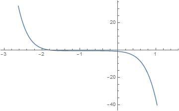
In accordance with Hayat et al. [15], Liao [18] and Akinbo and Olajuwon [19] suggestions, the non-zero auxiliary parameters hf, $\hbar_{\theta}$ and $\hbar_{\emptyset}$ play a crucial role in adjusting and controlling the convergence region of the series solution. Subject to the introduction of the following embedded parameters Ec=0.1, We=0.1, Mn=1, λT=0.1, λM=0.1, Pr=0.72, Sc=0.62, δ=1, R=0.1, Q=0.1 and S=0.2, the acceptable values of hf, $\hbar_{\theta}$ and $\hbar_{\emptyset}$ are chosen at a region where $\hbar-$ curve becomes parallel, such as $-1.4 \leq \hbar_{f} \leq-0.3$, $-1.5 \leq \hbar_{\theta} \leq-0.3$ and $-1.6 \leq h_{\emptyset} \leq-0.4$ (See Figures 2-4).
Figure 2. hf-curve of $f^{\prime \prime}(0)$ at 10th order of approximation
Figure 3. $\hbar_{\theta}$-curve of $\theta^{\prime}(0)$ at 10th order of approximation
Figure 4. $\hbar_{\emptyset}$ -curve of $\emptyset^{\prime}(0)$ at 10th order of approximation
Table 1 gives the details of the convergence of the iterations with the far field boundary conditions. As illustrated in the table, the momentum and concentration equations demonstrated quick convergence at 16th-order of iterations while the energy equations meet the unbounded domain at 26th-order of iterations.
Table 1. Convergence of solution
|
Order of Approximation |
$f^{\prime \prime}(0)$ |
$-\theta^{\prime}(0)$ |
$-\emptyset^{\prime}(0)$ |
|
5 |
-1.5210 |
0.4845 |
0.5412 |
|
10 |
-1.5209 |
0.4723 |
0.5341 |
|
12 |
-1.5208 |
0.4713 |
0.5337 |
|
14 |
-1.5208 |
0.4707 |
0.5336 |
|
16 |
-1.5207 |
0.4705 |
0.5335 |
|
18 |
-1.5207 |
0.4704 |
0.5335 |
|
20 |
-1.5207 |
0.4703 |
0.5335 |
|
22 |
-1.5207 |
0.4702 |
0.5335 |
|
24 |
-1.5207 |
0.4701 |
0.5335 |
|
26 |
-1.5207 |
0.4700 |
0.5335 |
|
30 |
-1.5207 |
0.4700 |
0.5335 |
|
We |
Mn |
λT |
λM |
Pr |
Sc |
Ec |
Q |
R |
S |
δ |
$R e_{x}^{\frac{1}{2}} C_{f}$ |
$R e_{x}^{-\frac{1}{2}} N u_{x}$ |
$R e_{x}^{-\frac{1}{2}} S h_{x}$ |
|
0.1 |
1.0 |
0.1 |
0.1 |
0.72 |
0.62 |
0.1 |
0.01 |
0.1 |
0.2 |
1.0 |
-1.856442 |
0.450873 |
0.533592 |
|
0.3 |
|
|
|
|
|
|
|
|
|
|
-2.114855 |
0.418395 |
0.506983 |
|
0.4 |
|
|
|
|
|
|
|
|
|
|
-2.580542 |
0.389764 |
0.484247 |
|
|
0.1 |
|
|
|
|
|
|
|
|
|
-1.247805 |
0.523830 |
0.575967 |
|
|
3.0 |
|
|
|
|
|
|
|
|
|
-2.970111 |
0.354152 |
0.483914 |
|
|
|
1.0 |
|
|
|
|
|
|
|
|
-1.182043 |
0.549533 |
0.591995 |
|
|
|
3.0 |
|
|
|
|
|
|
|
|
0.294860 |
0.657320 |
0.669378 |
|
|
|
|
1.0 |
|
|
|
|
|
|
|
-1.184597 |
0.549435 |
0.591925 |
|
|
|
|
3.0 |
|
|
|
|
|
|
|
0.298258 |
0.659895 |
0.671135 |
|
|
|
|
|
1.0 |
|
|
|
|
|
|
-1.860864 |
0.586667 |
0.531409 |
|
|
|
|
|
3.0 |
|
|
|
|
|
|
-1.874747 |
1.334314 |
0.526729 |
|
|
|
|
|
|
0.24 |
|
|
|
|
|
-1.847074 |
0.460574 |
0.282197 |
|
|
|
|
|
|
0.78 |
|
|
|
|
|
-1.859150 |
0.448428 |
0.627121 |
|
|
|
|
|
|
|
2.0 |
|
|
|
|
-1.848642 |
-0.335301 |
0.535973 |
|
|
|
|
|
|
|
4.0 |
|
|
|
|
-1.840715 |
-1.137066 |
0.538350 |
|
|
|
|
|
|
|
|
0.05 |
|
|
|
-1.854694 |
0.389698 |
0.534445 |
|
|
|
|
|
|
|
|
0.1 |
|
|
|
-1.851608 |
0.291237 |
0.535956 |
|
|
|
|
|
|
|
|
|
0.5 |
|
|
-1.861624 |
0.446613 |
0.763200 |
|
|
|
|
|
|
|
|
|
1.0 |
|
|
-1.865162 |
0.444121 |
0.965390 |
|
|
|
|
|
|
|
|
|
|
0.4 |
|
-2.726336 |
0.549444 |
0.613375 |
|
|
|
|
|
|
|
|
|
|
0.8 |
|
-5.951097 |
0.758515 |
0.784542 |
|
|
|
|
|
|
|
|
|
|
|
2.0 |
-1.856506 |
0.457345 |
0.533572 |
|
|
|
|
|
|
|
|
|
|
|
4.0 |
-1.856635 |
0.470294 |
0.533533 |
This section presents the dynamics of the different patients for better understanding of the study. The parameters are discussed by keeping Ra=0.7, Ec=1, We=0.1, Mn=1, Ps=1, λT=0.1, λM=0.1, Pr=0.72, Sc=0.62, δ=0.1, A=0.2, R=0.1 and Q=0.1, fixed for each varying parameter. The drag force effect is active on the surface due to the negative values of $\operatorname{Re}_{x}^{\frac{1}{2}} C_{f}$ which inturns impede the flow. However, the large values of Prandtl number (Pr), thermal and mass buoyancy parameter (λT,, λM) conttibutes to the enhancement of the Nusselt number $R e_{x}^{-\frac{1}{2}} N u_{x}$ and consequently improve the rate of heat transfer while the Sherwood number $R e_{x}^{-\frac{1}{2}} S h_{x}$ is strengthen for large values of Schmidt number (Sc), thermal and mass buoyancy parameter (λT,, λM). This inturn enhances the rate of mass transfer.
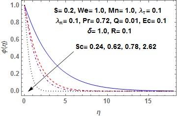
Figure 5. Temperature profile for different values of Sc
Figure 6. Temperature profile for different values of Pr
Figure 7. Velocity profile for different values of We
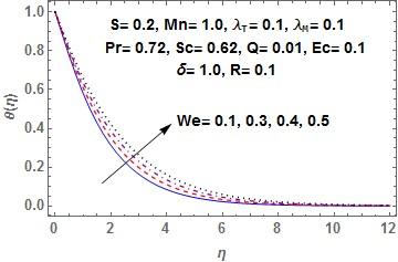
Figure 8. Temperature profile for different values of We
Figure 5 elucidates the effect of Schmidt number (Sc) on concentration profile. The diffusion properties of the fluid experiences greater fall for large values of Sc (due to the low molecular diffusivity). This inturns declines the concentration boundary layer thickness. Figure 6 presents the effect of Prandtl number (Pr) on temperature profile. It is noticed that increase in Pr due to low thermal diffusivity rapidly thins the temperature profile. However, this indicates that at small values of Pr, the fluid is highly conductive.
Figures 7-8 illustrate the behavior of Weissenberg number (We) on velocity and temperature profiles. Increase in We pioneer the effectiveness of the tensile stress which in turn steer-up the viscoelasticity impact across the boundary layer that consequently reduces the velocity of the fluid and momentum layer thickness. The reverse phenomenon is observed on temperature profile that ultimately strengthens the thermal layer thickness. Figures 9-10 present the behaviors of Magnetic Parameter (Mn) on velocity and temperature profiles. Obviously from Figure 9 due to the magnetic interaction, an electric field, produces a resistive forces called Lorentz force. This force acts against the flow and contract the velocity distribution and its layer thickness. Moreover, the reverse phenomenon is observed on temperature profile due to the frictional heating with the impact of the Lorentz, thereby improves the thermal boundary layer thickness.
Figure 9. Velocity profile for different values of Mn
Figure 10. Temperature profile for different values of Mn
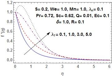
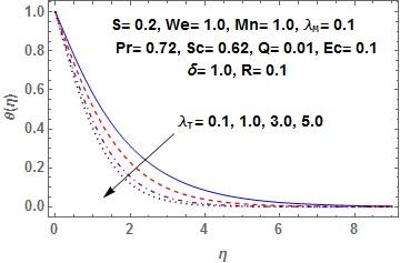
The presence of thermal and mass buoyancy parameters (λT,, λM) accelerate the motion of the fluid as shown in Figure 11 and Figure 13. These in turn improves the momentum layer thickness. However, reverse phenomenon is observed on temperature and concentration which consequently declines the thermal and concentration boundary layers thicknesses as shown in Figure 12 and Figure 14 respectively.
Figure 11. Velocity profile for different values of λT
Figure 12. Temperature profile for different values of λT
Figure 13. Velocity profile for different values of λM
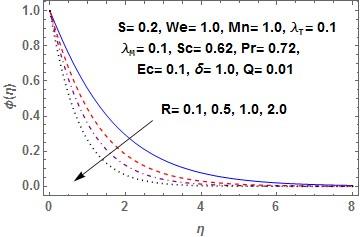
Figure 15 describes the behavior of internal heat generation (Q) on temperature profile. Large values of Q magnifies the random movement of the fluid molecules which in turns energies the temperature profile and thermal boundary layer thickness. Figure 16 depicts the behaviors of Eckert number (Ec) on temperature profile. However, the temperature of the fluid improves with the enhancement in viscous dissipation, since the heat energy is stored in the fluid due to frictional heating which consequently boosts thermal layer thickness. Figure 17 reveals the effect of chemical reaction (R) on concentration profile. Large values of R deteriorates the concentration buoyancy effect of which the resulting effect thins the concentration profile as well as its layer thickness.
Figure 14. Concentration profile for different values of λM
Figure 15. Temperature profile for different values of Q
Figure 16. Temperature profile for different values of Ec
The presence of Suction parameter (S>0) moves the motion of the fluid, temperature distribution as well as concentration of the fluid towards the boundary as shown in Figures 18-20. This inturns lower their layers thicknesses. It is noteworthy that the porous stretching sheet of this type with suction beneath it is sometimes used to prevent the boundary layer from separating (see Hayat et al. [15]).
Figure 17. Concentration profile for different values of R
Figure 18. Velocity profile for different values of S
Figure 19. Temperature profile for different values of S
Figure 20. Concentration profile for different values of S
In this article, Computational investigation of Heat and Mass Transfer on MHD Walters’ B Fluid over a vertical stretching Surface with Suction\Injection has been studied. The problem is solved by HAM at 20th-order of approximation due to the unbounded domain to meet the far field boundary condition and the parameters encountered are discussed accordingly with the following conclusions.
· The enhancement in Magnetic field pioneer frictional heating which in turns strengthen the thermal layer
· The non-Newtonian properties is possessing in the presences of Weissenberg number, with the great industrial application such as plastic film, artificial fibers and higher molecular-weight liquid used in Science discipline.
· Large values of thermal and mass buoyancy parameters accelerate the motion of the fluid while higher values of internal heat generation magnifies the random movement of the fluid molecules which in turns energies the operating temperature and enable penetration of thermal effect to the quiescent fluid.
· Large values of Prandtl number due to low thermal diffusivity contributes to the falling of the temperature across the layer, indicating that at small values of Prandtl number, the fluid is highly conductive.
The authors would like to thank the reviewers and anonymous referees for their useful suggestions that led to definite improvement in the paper.
|
W |
Weissenberg number |
|
M |
Magnetic field parameter |
|
Pr |
prandtl number |
|
Ec |
Eckert number |
|
β |
Reaction rate parameter |
|
Q |
Heat Absorption parameter |
|
λT |
Thermal buoyancy parameter |
|
λM |
Mass buoyancy parameter |
|
Sc |
Schmidt number |
|
Q |
Heat Absorption parameter |
|
Greek symbols |
|
|
η |
Similarity variable |
|
ψ |
Stream function |
[1] Iqbal, Z., Mehmood, Z., Ahmad, B. (2017). Elastic deformation analysis on MHD viscous dissipative flow of viscoelastic fluid: An exact approach. Communications in Theoretical Physics, 67(5): 561-568. https://doi.org/10.1088/0253-6102/67/5/561
[2] Mahapatra, T.R., Dholey, S., Gupta, A.S. (2007). Momentum and heat transfer in the magnetohydrodynamic stagnation-point flow of a viscoelastic fluid toward a stretching surface. Meccanica, 42(3): 263-272. https://doi.org/10.1007/s11012-006-9040-8
[3] Nadeem, S., Rashid, M., Noreen, S.A. (2014). Thermo-diffusion effects on MHD oblique stagnation-point flow of a viscoelastic fluid over a convective surface. The European Physical Journal Plus, 129: 182. https://doi.org/10.1140/epjp/i2014-14182-3
[4] Ariel, P.D. (2008) Two dimensional stagnation point flow of an elastico-viscous fluid with partial slip. Journal of Applied Mathematics and Mechanics, 88(4): 320-324. https://doi.org/10.1002/zamm.200700041
[5] Hayat, T., Kiyani, M.Z., Ahmad, I., Khan, M.I., Alsaedi, A. (2018). Stagnation point flow of viscoelastic nanomaterial over a stretched surface. Results in Physics, 9: 518-526. https://doi.org/10.1016/j.rinp.2018.02.038
[6] Poonia, M., Bhargava, R. (2015). Finite element solution of oblique stagnation-point flow of viscoelastic fluid and heat transfer with variable thermal conductivity. International Journal of Computing Science and Mathematics (IJCSM), 6(6): 519-537. https://doi.org/10.1504/IJCSM.2015.073578
[7] Reza, M., Panigrahi, S., Mishra, A.K. (2017). Stagnation point flow and heat transfer for a viscoelastic fluid impinging on a quiescent fluid. Sadhana, 42(11): 1979-1986. https://doi.org/10.1007/s12046-017-0739-0
[8] Bariş, S. (2003). Steady three-dimensional flow of a second grade fluid towards a stagnation point at a moving flat plate. Turkish Journal of Engineering and Environmental Sciences, 27(1): 21-29.
[9] Qayyum, S., Hayat, T., Shehzad, S.A., Alsaedi, A. (2017). Effect of a chemical reaction on magnetohydrodynamic (MHD) stagnation point flow of Walters-B nanofluid with newtonian heat and mass conditions. Nuclear Engineering and Technology, 49(8): 1636-1644. https://doi.org/10.1016/j.net.2017.07.028
[10] Ahmad, I. (2013). On unsteady boundary layer flow of a second grade fluid over a stretching sheet. Advances in Theory Applied Mechanics, 6(2): 95-105. https://doi.org/10.12988/atam.2013.231
[11] Sadeghy, K., Sharifi, M. (2004). Local similarity solution for the flow of a second grade viscoelastic fluid above a moving plate. International Journal of NonLinear Mechanics, 39(8): 1265-1273. https://doi.org/10.1016/j.ijnonlinmec.2003.08.005
[12] Ayub, M., Zaman, H., Sajid, M., Hayat, T. (2008). Analytical solution of stagnation-point flow of a viscoelastic fluid towards a stretching surface. Communications in Nonlinear Science and Numerical Simulation, 13(9): 1822-1835. https://doi.org/10.1016/jcnsns.2007.04.021
[13] Chen, C.H. (2010). On the analytic solution of MHD flow and heat transfer for two types of viscoelastic fluid over a stretching sheet with energy dissipation, internal heat source and thermal radiation. International Journal of Heat and Mass Transfer, 53(19): 4264-4273. https://doi.org/10.1016/j.ijheatmasstransfer.2010.05.053
[14] Nandeppanavar, M.M., Vajravelu, K., Abel, M.S. (2011). Heat transfer in MHD viscoelastic boundary layer flow over a stretching sheet with thermal radiation and non-uniform heat source/sink. Communications in Nonlinear Science and Numerical Simulation, 16(9): 3578-3590. https://doi.org/10.1016/j.cnsns.2010.12.033
[15] Hayat, T., Asad, S., Mustafa, M., Hamed, H.A. (2014). Heat transfer analysis in the flow of Walters’ B fluid with a convective boundary condition. Chinese Physics B, 23(8): 084701-7. https://doi.org/10.1088/1674-1056/23/8/084701
[16] Akinbo, B.J., Olajuwon, B.I. (2019). Convective heat and mass transfer in electrically conducting flow past a vertical plate embedded in a porous medium in the presence of thermal radiation and thermo diffusion. Computational Thermal Sciences, 11(4): 367-385. https://doi.org/10.1615/ComputThermalScien.2019025706
[17] Akinbo, B.J., Olajuwon, B.I. (2019). Homotopy analysis investigation of heat and mass transfer flow past a vertical porous medium in the presence of heat source. International Journal of Heat and Technology, 37(3): 899-908. https://doi.org/10.18280/ijht.370328
[18] Liao, S.J. (2003). Beyond perturbation: an introduction to Homotopy Analysis Method. Chapman and Hall, Boca Raton, Fla., USA.
[19] Akinbo, B.J., Olajuwon, B.I. (2019). Heat and mass transfer in magnetohydrodynamics (MHD) flow over a moving vertical plate with convective boundary condition in the presence of thermal radiation. Sigma Journal of Engineering & Natural Sciences, 37(3): 1031-1053.