Yanán Camaraza-Medina* | Andres A. Sánchez-Escalona | Yoalbys Retirado-Mediaceja | Osvaldo F. García-Morales
OPEN ACCESS
At present day, the use of Air Cooled Condenser (ACC) in power plants is a trend in regions with difficult access to water. In the available literature the performance analysis of the ACC is a difficult task, because not have an only method that includes all of the elements related to the ACC's use and his effect on the power plant. The Kröger's method is recognized as the more effective for the thermal analysis of the ACC, but this procedure not offer satisfactory results for elevated values of environmental temperature, as it is the case of Cuba. In the present work is developed a unique method of analysis that considers the effect of the environmental variables on the ACC, allowing obtaining its final effect on the condenser facilities. The new proposal follows the same logical order shown in the Kröger's method, since it is the one with the greatest acceptance and dissemination among researchers and specialists working in this field. In this new method are considered news procedures for the estimation of the average heat transfer coefficient, pressure drop and thermal assessment.
efficiency, power plant, sugar industry, heat transfer
At the present time, the deficit of water and the eminence of the use of alternative energy sources have generated innumerable efforts to solve the existing insufficiencies in the known technologies. The use of the biomass as energetic source for electric power generation has been one of the alternatives of bigger acceptance in regions with agricultural and wooded potential [1, 2].
In order to reduce the water consumption in power plants, a technology that wins adepts at the present time is the dry condensation, because, as his name suggests, reduce the water consumption perceptibly in the operation, achieving rates of disuse close to 95% regarding wet condensers. The Air Cooled Condenser (ACC) is the dry condenser preferred, being known already and used in Biomass Power Plant (BPP) in countries as United States, Turkey, China, Malaysia, India, South Africa, Germany and Spain [3, 4].
In Cuba has been planned for the five-year period (2020-2025) a big investment that will allow to the installation of 1650 MW with the use of renewable energy, (24% of the country consumption). Of this volume, 875 MW will be produced by 25 BPP associated to equal numbers of sugarcane processing plant (SPP), that will supply bagasse to be used as biomass, while the BPP supplies the vapor required by the industrial process of the SPP [5].
In Cuba, the National Institute of Hydraulic Resources (NIHR) confirmed that the last five-year period (2015-2019), the deficit valued of water has increased in a 12 percent, declaring in the hydrological bulletin 03-2020 a total of 57 water basins in critical state. This situation generated the approval of the law 24/2017 and the decree 337/2017 about the use of the earthly waters, becoming regulated of strict way the water use in basins in state critical, of the foreseen BPP, a total of 17 are placed in suchlike zones. Considering the confirmed deficit of water and the potentiality of the use of the biomass as energetic source, the use of ACC can be an effective solution [1-3].
Cuba is not distant of the global crisis of water; therefore, it is essential to give an adequate use, this has motivated that has been considered to medium term the use of technology ACC in the projects planned of BPP [2, 3].
At the present time, the performance analysis of the ACC is a difficult task, because not have an only method that includes all of the elements related to the ACC's use and his effect on the BPP. In the available literature recognizes the Kröger's method as the more effective for the thermal analysis of the ACC, being highly influenced by the temperature of dry bulb (TTBS). However, the climatic characteristics of Cuba, with a high value of (TTBS), do not enable an effective use of this method of analysis. The results obtained by this procedure present a high level of dispersion, finding real cases with average errors of the 60% [6, 7].
In order to eliminate the combination fractioned of methods, used at the present time in the related evaluation of ACC and the high values of dispersion, the authors aims to as central objective in the present investigation, the development of an only method of analysis more precise that the current procedures and that besides includes the influence of the environmental variables on the ACC. The elements shown in this paper are a part of the post-doctoral investigation accomplished by the main author [6-8].
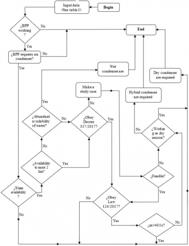
2.1 Basic methodology for the selection of the condenser more adequate
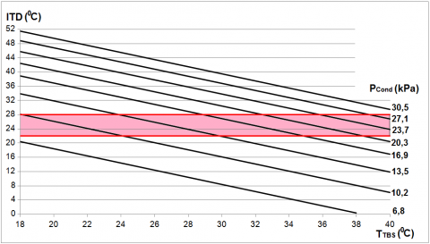
For the selection of the most adequate condenser, the methodology given in the Figure 1 was applied. For this purpose is required to have a group of primary parameters, which are summarized in the Table 1. The diagram of utilization (see Figure 2) is a fast application method, very used to verify the effectiveness use of the ACC in pre-established operating conditions.
In the diagram of utilization an interaction between the initial temperature difference (ITD) and the temperature of dry bulb (TTBS) are shown, in terms of the steam pressure in the turbine outlet (PCond). The zone recommended of favorable operation was obtained in recent investigations, being shady in pink in the Figure 2 [9].
Figure 1. Selection of the more adequate condenser for BPP
The initial temperatures difference (ITD) is obtained as, [10]:
$\mathrm{ITD}=\mathrm{T}_{\mathrm{EntVapor}}-\mathrm{T}_{\mathrm{TBS}}$ (℃) (1)
In Eq. (1) TEntVapor is the fluid temperature in the condenser outlet, in ℃.
Table 1. Initial parameters required for the ACC evaluation
|
- |
Availability of water for the condenser |
|
PC |
Plant capacity |
|
- |
Availability of space for the facility |
|
- |
Cost for the water use, in USD⁄m3 |
|
- |
Availability of biomass and electric lines. |
|
- |
Towns and roads near |
|
- |
Altitude above sea level |
|
hrel |
Relative humidity, in %. |
|
TTBS |
Temperature of dry bulb, in ℃ |
|
VV |
Velocity of the wind, in km/h |
|
TAD |
Unloading temperature permitted in the water reservoirs, in ℃ |
Figure 2. Diagram of utilization
2.2 Basic methodology for the selection of the condenser more adequate
The proposal methodology follows the same logical order shown in the Kröger's method, since it is the one with the greatest acceptance and dissemination among researchers and specialists working in this field. In this new method are considered news procedures for the estimation of the average heat transfer coefficient, pressure drop and thermal assessment of the ACC. The proposed procedure is described step to step of the following manner:
1- Define the initial required variables (see Table 1)
2- Determine the ideal pressure of the vapor in the turbine outlet, (see Table 2).
Table 2. Ideal pressure of the vapor in the turbine outlet
|
Interval of wind velocity |
Ideal outlet pressure (kPa) |
|
|
$0 \leq V_{v}<6.4 \mathrm{km} / \mathrm{h}$ |
$\mathrm{P}_{\text {Back }}=17.5 \ln \left(\mathrm{T}_{\mathrm{TBS}}\right)-45.3$ |
(2) |
|
$6.4 \leq V_{V}<12.8 \mathrm{km} / \mathrm{h}$ |
$P_{B a c k}=22 \ln \left(T_{T B S}\right)-58.2$ |
(3) |
|
$12.8 \leq V_{v}<19.2 \mathrm{km} / \mathrm{h}$ |
$\mathrm{P}_{\text {Back }}=22.9 \ln \left(\mathrm{T}_{\mathrm{TBS}}\right)-60.4$ |
(4) |
|
$19.2 \leq V_{v}<25.6 \mathrm{km} / \mathrm{h}$ |
$\mathrm{P}_{\mathrm{Back}}=22.1 \ln \left(\mathrm{T}_{\mathrm{TBS}}\right)-56.9$ |
(5) |
|
$25.6 \leq V_{V}<32.0 \mathrm{km} / \mathrm{h}$ |
$P_{B a c k}=21.8 \ln \left(T_{T B S}\right)-55.2$ |
(6) |
|
$V_{V} \geq 32.0 \mathrm{km} / \mathrm{h}$ |
$P_{B a c k}=22.7 \ln \left(T_{T B S}\right)-57.1$ |
(7) |
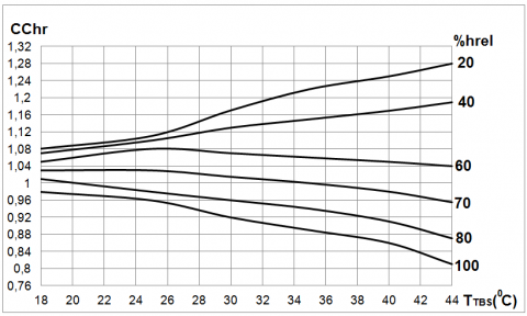
3- Define the correcting factors for the effect of the wind (Crec) and relative humidity (CChr), see Figures 3 and 4.
4- Determine the real pressure of the vapor in the turbine outlet.
$P_{S T}=P_{B a c k} \cdot C_{r e c} \cdot C C h r \quad(k P a)$ (8)
Figure 3. Correcting factors for the effect of the wind
Figure 4. Correcting factors for the effect of the relative humidity
5- Define the vapor production of the steam boiler $\mathrm{m}_{\mathrm{I}}$ , the rate of vapor in the intermediate extraction $\mathrm{m}_{\mathrm{E}}$ and the flow at the turbine outlet magua.
6- Obtain the thermodynamic properties (enthalpy and entropy) in the turbine inlet (hI; sI) and intermediate extraction in the turbine, (hE; sE).
7- Establish the required initial variables of the combined process, (see Table 3).
Table 3. Initial required variables of the combined process
|
Initial required variables |
unit |
|
SPP mill capacity |
t/h |
|
BPP capacity |
MW |
|
Temperature of the vapor at steam boiler outlet |
℃ |
|
Temperature of the water supply to the steam boiler |
℃ |
|
Vapor temperature at intermediate extraction in the turbine. |
℃ |
|
Pressure of the vapor at steam boiler outlet |
MPa |
|
Pressure of the vapor at intermediate extraction in the turbine. |
MPa |
|
Pressure of the water supply to the steam boiler |
MPa |
|
Vapor rate at intermediate extraction in the turbine. |
kg/s |
|
Elementary composition of the biomass |
% |
8- Calculate the useful power in the turbine installation, using the following Equation:
$W_{\text {Elec}}=\left[\begin{array}{c}
m_{\text {agua}} \cdot\left(h_{I}-h_{E}\right)+ \\
+\left(m_{\text {agua}}-m_{E}\right) \cdot\left(h_{I}-h_{E}\right)
\end{array}\right] \cdot \eta_{\text {em}} \cdot \eta_{r i}$ (9)
In Eq. (9) ηem and ηri is the electromechanical and relative internal performance of the turbine respectively.
9- Obtain the thermodynamic properties of the vapor in the turbine outlet, (see Table 4).
Table 4. Thermodynamic properties required, turbine outlet
|
hcond |
Enthalpy |
kJ⁄kg |
|
scond |
Entropy |
kJ⁄(kg∙℃) |
|
Th |
Temperature of the vapor |
℃ |
|
PrL |
Prandtl number for single-phase |
- |
|
μL |
Liquid dynamic viscosity |
kg⁄(m∙s) |
|
μV |
Steam dynamic viscosity |
kg⁄(m∙s) |
|
ρL |
Liquid density |
kg⁄m3 |
|
ρV |
Steam density |
kg⁄m3 |
|
λL |
Fluid thermal conductivity |
W⁄(m∙℃) |
|
CpL |
Liquid specific heat |
kJ⁄(kg∙℃) |
10- Define the tube arrangements and the transverse pitch ST and longitudinal pitch SL measured between tube centers, in m.
11- Define characteristics of the fin tubes (all the dimensions will be given in meters), which include, di and de is the inner and outer diameter of the bare tube (without fins), fins height ha, fins thicknessea, wall thickness of the tube eT, tube length $1$ and number of fins per linear meter of tube Fa.
12- Assume a global coefficient of heat transfer K, in the range of values K1=30 to 100 W⁄(m2∙℃).
13- Define in a first approximation the condensed outlet temperature in the ACC by means of the following Equation:
$\mathrm{T}_{\mathrm{scond}}=\left(\mathrm{T}_{\mathrm{EntVapor}}+\mathrm{T}_{\mathrm{TBS}}\right) / 2\left({ }^{\circ} \mathrm{C}\right)$ (10)
14- Calculate the initial temperatures difference (ITD) with the use of the Equation (1).
15- Check in the Figure 2 if ITD values are located in the recommended zone, otherwise taking a value between ITD=22 to 28 ℃.
16- Determine the Logarithmic Mean Temperature Difference (LMTD) in the ACC, by means of the following Equation:
$\mathrm{LMTD}=\frac{\mathrm{ITD}-\mathrm{TTD}}{\ln \left(\frac{1 \mathrm{TD}}{\mathrm{TTD}}\right)}$ (℃) (11)
In Equation (11) $TTD$ is the temperature difference of the flow in the the condensed side, in ℃.
17- Obtain the thermodynamic properties in the ACC outlet, enthalpy hfluid (in kJ/kg) and entropy sfluid, in kJ⁄(kg∙℃).
18- Determine the transferred heat in the ACC by the following Equation:
$\mathrm{Q}=\mathrm{m}_{\text {agua }} \cdot\left(\mathrm{h}_{\text {cond }}-\mathrm{h}_{\text {fluid }}\right)(\mathrm{kW})$ (12)
19- Obtain the heat transfer surface of a single fin (in $\mathrm{m}^{2}$ by the following Equation:
$A_{\mathrm{a}}=\pi \mathrm{e}_{\mathrm{a}}\left(\mathrm{d}_{\mathrm{e}}+2 \mathrm{h}_{\mathrm{a}}\right)+2 \pi\left[\left(\frac{\mathrm{d}_{\mathrm{e}}}{2}+\mathrm{h}_{\mathrm{a}}\right)^{2}-\left(\frac{\mathrm{d}_{\mathrm{i}}}{2}\right)^{2}\right]$ (13)
20- Define the fins number per tube.
$\mathrm{n}_{\mathrm{aT}}=\mathrm{F}_{\mathrm{a}} \cdot \mathrm{l}$ (14)
21- Determine the heat transfer surface of and finned tube. by the following Equation:
$A_{T}=\pi d_{e} \cdot\left(l-e_{a} n_{a T}\right)+A_{a} n_{a T} \quad\left(m^{2}\right)$ (15)
22- Determine the inner surface of the fiined tube:
$A_{I}=\pi \cdot l \cdot\left(d_{e}-2 e_{T}\right) \quad\left(m^{2}\right)$ (16)
23- Obtain the necessary heat transfer for the ACC, using the following Equation:
$\mathrm{F}=\mathrm{Q} /\left(\mathrm{LMTD} \cdot \mathrm{K}_{1}\right) \quad\left(\mathrm{m}^{2}\right)$ (17)
23- Determine the number of tubes that would have the ACC in a first approximation, using the following Equation:
$n_{\text {tubos }}=F /\left(A_{T} \cdot A_{I}\right)$ (18)
23- Calculate the liquid and vapor Reynolds number, using the following Equations [11, 12]:
$\mathrm{Re}_{\mathrm{L}}=\frac{\mathrm{m}_{\mathrm{agua}} \cdot(1-\mathrm{x}) \cdot \mathrm{d}_{\mathrm{i}}}{\mu_{\mathrm{L}} \cdot 0.785 \cdot \mathrm{d}_{\mathrm{i}}^{2} \cdot \mathrm{n}_{\mathrm{tubos}}}$ (19)
$\operatorname{Re}_{\mathrm{V}}=\frac{\mathrm{m}_{\mathrm{agua}} \cdot \mathrm{x} \cdot \mathrm{d}_{\mathrm{i}}}{\mu_{\mathrm{V}} \cdot 0.785 \cdot \mathrm{d}_{\mathrm{j}}^{2} \cdot \mathrm{n}_{\mathrm{tubos}}}$ (20)
In Eqns. (19) and (20), X is the thermodynamic vapor quality.
24- Calculate the heat transfer coefficient in the inner portion of the tube and the drop pressure by means of the procedure gived in [6, 7].
25- Determine the thermodynamic properties of the air at TTBS, (see Table 5).
Table 4. Thermodynamic properties required, ACC inlet in the air side
|
ha |
Enthalpy |
kJ⁄kg |
|
sa |
Entropy |
kJ⁄(kg∙℃) |
|
Pra |
Prandtl number |
- |
|
μa |
Dynamic viscosity |
kg⁄(m∙s) |
|
ρa |
Density |
kg⁄m3 |
|
λa |
Thermal conductivity |
W⁄(m∙℃) |
|
Cpa |
Specific heat |
kJ⁄(kg∙℃) |
26- Determine the enthalpy of the air at ACC outlet has by air side, in kJ⁄kg.
27- Calculate the airflow necessary, as:
$\mathrm{m}_{\mathrm{aire}}=\mathrm{Cp}_{\mathrm{a}}\left(\mathrm{T}_{\mathrm{SACC}}-\mathrm{T}_{\mathrm{TBS}}\right) \quad(\mathrm{kg} / \mathrm{s})$ (21)
In Eq. (21) $\mathrm{T}_{\mathrm{SACC}}$ is the air temperature at ACC outlet.
28- Calculate the initial air velocity as:
$\mathrm{V}_{\mathrm{n}}=\mathrm{m}_{\text {aire }} /\left(75.6 \cdot \mathrm{n}_{\text {vent }}\right) \quad(\mathrm{m} / \mathrm{s})$ (22)
In Eq. (22) nvent is the number of fans used in the ACC, for a first aproximation take nvent=1.
29- Calculate the maximum fluid velocity of the air in the tube bank.
30- Calculate the heat transfer coefficient in the air side portion and the drop pressure by means of the procedure gived in [5].
31- Determine the thermal resistances in the ACC.
32- Determine the thermal efficiency of an single fin, ηA.
33- Determine the performance of the extended surface as:
$\eta_{\mathrm{W}}=1-\mathrm{n}_{\mathrm{aT}} \mathrm{A}_{\mathrm{a}}\left(1-\mathrm{n}_{\mathrm{aT}}\right) /\left(\mathrm{A}_{\mathrm{T}} \cdot \mathrm{n}_{\mathrm{tubos}}\right)$ (23)
34- Determine the global heat transfer K2.
35- Compare the global coefficients K2 and K1. If the average error EE is lower than 5% the values K2.are acepted, otherwise, is necessary to repeat the study from the point 12 with the new value of the global heat transfer coefficient K2. The average error EE is obtained as:
$\mathrm{E}_{\mathrm{E}}=100 \cdot\left|\frac{K_{2}-K_{1}}{K_{2}}\right|$ (%) (24)
36- Obtain the real heat transfer surface $\mathrm{F}^{\prime}$ required by the ACC as:
$\mathrm{F}^{\prime}=\mathrm{Q} /\left(\mathrm{LMTD} \cdot \mathrm{K}_{2}\right) \quad\left(\mathrm{m}^{2}\right)$ (25)
37- Determine the cost of ecological trace, in USD⁄(GJ∙year), for the estimated emissions associated to the use of AAC as:
$G_{E m i s}=(6.02-0.434 B) \cdot A \cdot e^{0.226 B}$ (26)
In Eq. (26) e is de Euler constant value, while A and B are constants values, conditioned to the emission of greenhouse effect gases. Values of constant A and B are obtained as [13]:
$A=\ln \left[\left(C O_{2}\right)^{0.1} \cdot S O_{2}\right]^{0.1}+0.252$ (27)
$B=\log \left[\frac{\left(C H_{4} \cdot N O_{X} \cdot(C O)^{0.04}-(S O)^{2}\right)^{2}}{N_{2} O}\right]$ (28)
In Eqns. (27) and (28) the volumes of polluting gases are given in Gg.
In this paper the methods developed for the analysis of the average coefficients of heat transfer are integrated to the proposed procedure. The shown material details gradually, the logical sequence to follow in the thermal evaluation of the ACC that operates coupled to a BPP.
The results obtained with the application of the method proposed to case studies, find coincidence between the obtained values and the reported values available in the literature specialized on the subject.
The presented method allows facilitating the analysis and eludes to come to fractioned procedures to evaluate an ACC. In the calculation of the average heat transfer coefficients are applied new methods of analysis, that allow decreasing the index of uncertainty with respect to methods known at the present time and reduces the dispersion in the final results. Finally,are presented the basics element required for the estimation of the ecological step associated to emissions of greenhouse effect gases, due to the use of ACC.
[1] Camaraza-Medina, Y., Cruz-Fonticiella, O.M., García-Morales, O.F. (2017). Element for the Estimation of Thermodynamic Properties of Cane and Forest Biomass. Revista Ciencias Técnicas Agropecuarias, 26(4): 76-82.
[2] Camaraza-Medina, Y., Cruz-Fonticiella, O.M., Garcia-Morales, O.F. (2018). Obtención de un modelo para la determinación del coeficiente medio de transferencia de calor por condensación en sistemas ACC. Tecnología Química, XXXVIII(1): 230-246.
[3] Camaraza, Y. (2017). Introducción a la termo transferencia. Editorial Universitaria, La Habana, 515-535.
[4] Camaraza-Medina, Y., Cruz-Fonticiella, O.M., García-Morales, O.F. (2018). Predicción de la presión de salida de una turbina acoplada a un condensador de vapor refrigerado por aire. Centro Azúcar, 45(1): 50-61.
[5] Camaraza-Medina, Y., Rubio-Gonzales, A.M., Cruz-Fonticiella, O.M., Garcia-Morales, O.F. (2018). Simplified analysis of heat transfer through a finned tube bundle in air-cooled condenser. MMEP, 5(3): 237-242. https://doi.org/10.18280/mmep.050316
[6] Camaraza-Medina, Y., Hernandez-Guerrero, A., Luviano-Ortiz, J.L., Cruz-Fonticiella, O.M., García-Morales, O.F. (2019). Mathematical deduction of a new model for calculation of heat transfer by condensation inside pipes. International Journal of Heat and Mass Transfer, 141: 180-190. https://doi.org/10.1016/j.ijheatmasstransfer.2019.06.076
[7] Camaraza-Medina, Y., Hernández-Guerrero, A., Luviano-Ortiz, J.L., Mortensen-Carlson, K., Cruz-Fonticiela O.M., García-Morales, O.F. (2019). New model for heat transfer calculation during film condensation inside pipes. International Journal of Heat and Mass Transfer, 128: 344-353. https://doi.org/10.1016/j.ijheatmasstransfer.2018.09.012
[8] Medina, Y.C., Khandy, N.H., Fonticiella, O.M.C., Morales, O.F.G. (2017). Abstract of heat transfer coefficient modelation in single-phase systems inside pipes. Mathematical Modelling of Engineering Problems, 4(3): 126-131. https://doi.org/10.18280/mmep.040303
[9] Sagastume-Gutiérrez, A., Cabello-Eras, J.J., Hens, L., Vandecasteele, C. (2018). Data supporting the assessment of biomass based electricity and reduced GHG emissions in Cuba. Data in Brief, 17: 716-723. https://doi.org/10.1016/j.dib.2018.01.071
[10] Suárez, J.A. (2019). Energy, environment and development in Cuba (original text In Spanish), Editorial Oriente, Santiago de Cuba, Cuba, 124-177.
[11] http://www.one.cu/aec2019.htm, accessed on April.3, 2020.
[12] Medina, Y.C., Fonticiella, O.M.C., Morales, O.F.G. (2017). Design and modelation of piping systems by means of use friction factor in the transition turbulent zone. Mathematical Modelling of Engineering Problems, 4(4): 162-167. https://doi.org/10.18280/mmep.040404
[13] Camaraza-Medina, Y. (2020). Current Trends in Cuba on the Environmental Impact and Sustainable Development. Tecnica Italiana-Italian Journal of Engineering Science, 64(1): 103-108. https://doi.org/10.18280/ti-ijes.640116