OPEN ACCESS
The Stirling engine design process is mostly focused on the study of the engine regenerator, whose thermal efficiency is strictly related to the global efficiency of the engine.
The present work aims to setup a numerical model by means of OpenFOAM libraries to simulate the engine regenerator as a porous media, in order to reduce the overall computational cost of the simulations and to obtain a suitable model that can be eventually used for topological optimization. The solid part of the numerical domain, i.e. the stoked wires, is represented as a zone with the highest porosity, whereas intermediate areas are defined in order to simulate the boundary layers in proximity of the walls. The presence of porous media is modelled by introducing a Darcy-type pressure drop in the momentum equation, whereas in the energy equation the thermal properties of the solid, intermediate and fluid materials are modelled by means of a linear function of the porosity value in the domain.
After a process of tuning, the results obtained with this model are reported for different flow conditions in terms of both aerodynamic and thermal performances, thus showing a good agreement with the numerical results obtained with a more classical CFD methodology.
Stirling engine, CFD, porous media, regenerator
In the field of energy generation and heating/cooling systems, a promising alternative to steam engines and internal combustion engines is represented by Stirling engines. This engine is classified as an external combustion engine, characterized by high reliability and robustness. The main advantages of such an engine are the possibility of using compressible flow, i.e. air, as working fluid and any type of heat source (e.g. gas coal, concentrated solar heat). On the other hand, only a low specific power is achievable with this type of technology.
Most of the studies on the Stirling engine focuses on analyzing the performance of a single component: the heat exchanger located between the hot and cold streams, also referred to as the engine regenerator. Indeed, it is reported that the main influence on the Stirling engine efficiency is given by the regenerator performances. The engine regenerator role is to store the thermal heat taken from the hot stream and to release it to the cold stream, in order to increase the thermal efficiency of the whole system [1]. The efficiency of such a component can reach extremely high values under specific conditions, close to unit, as shown in the work of Tanaka et al. [2], which analyses the performance of a regenerator within laminar regime and by using an oscillating flow. In the design process of such a component, it is required to reduce the pressure losses through the component as much as possible, without reducing the thermal efficiency.
The regenerator is generally composed by matrices of metallic wires, with different configurations in order to improve the performance of the system in terms of both heat exchange and aerodynamic behavior.
Because of the increasing interest on the Stirling engine technology, several studies have been performed on different configurations in order to evaluate their performance, both experimentally [3,4] and numerically. In the numerical studies, two main approaches are found. The first consists in modelling the wires as walls and simulating one element of the matrix, by evaluating the behavior of the flow passing through the wires, as reported in the works of Costa et.al. [5,6], Faruoli et al. [7] and Bello et al. [8], where the fluid-dynamic and the thermal performances are computed in terms of friction coefficient, thermal efficiency and Nusselt number. The second approach defines the matrix as a porous block with a porosity that enables to simulate the flow behavior of the actual geometry. This approach is used in the literature to study heat exchangers [9], and, more specifically, is employed for the Stirling engine regenerator [1, 10, 11].
The use of a porous media block to represent the wire matrices approximates the actual behavior of the Stirling regenerator. Indeed it enables to reproduce the overall flow behavior and, consequently, to evaluate the component performances even if it does not allow to analyse the details of the flow distribution inside the domain. On the other side, it allows to reduce the overall computational cost, by using regular, structured computational grid. Moreover, the model can be eventually used for a topological optimization process [12].
In this work, a novel numerical approach is used where the wires are represented as fully solid material, whereas the surrounding regions are represented as fully fluid. This strategy enables to characterize the flow behavior locally other than the macroscopic parameters that correspond to the performances of the regenerator. The development of the model that describes the regenerator geometry as a porous zone, under different flow conditions, is given. The model has been implemented within the OpenFOAM framework. Then, the model is applied to the regenerator configuration studied by Bello et al. [8]. Finally, the results of these simulations are compared with those obtained with a more classical Computational Fluid Dynamics (CFD) approach.
2.1 Computational domain
The analysis of the Stirling regenerator focuses on the characterization of the flow behavior through its wires. Indeed, the regenerator is made by matrices of wires netting stacked next, or on top, of each other.
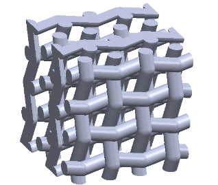
Specifically, the configuration studied in this work is a misaligned wires distribution that is also employed by Bello et al. [8] as optimal configuration in their study (Figure 1).
Figure 1. Regenerator matrix configuration
The domain considered is 3D, consisting of a parallelepiped with a cross-section of 1 mm × 1 mm and a total length of 5 mm. The wire matrix is placed 2 mm downstream the inlet section, and it has a length, L, of 0.922 mm. The wire matrix is characterized by the definition of the porosity, πv and of the hydraulic diameter, dh, defined in Eq. 1 and Eq. 2, respectively:
${{\pi}_{v}}=\frac{{{V}_{tot}}-{{V}_{m}}}{{{V}_{tot}}}$ (1)
${{d}_{h}}=\frac{4{{\pi}_{v}}}{\phi (1-{{\pi }_{v}})}$ (2)
In the equations Vtot is the total volume of the matrix and Vm is the volume occupied by the wires, Φ is the ratio between the surface area and the volume of the woven matrix. The values of these parameters for the geometry under investigation are reported in Table 1.
Table 1. Geometrical properties of the regenerator
|
L |
dh |
πv |
|
0.922 m |
0.172 mm |
0.641 |
In this work, a different approach is used since the wires are modelled as zones of porous material, by considering the porosity as the fluid volume fraction, ε, defined for each cell as:
$\varepsilon\text{=}\frac{volume\text{ }of\text{ }fluid}{total\text{ }volume}$
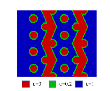
The topology of the numerical domain is set by considering the wires as fully solid zone, thus characterized by a value ε=0, whereas the rest of the domain is considered as fully fluid, with an imposed value ε=1. With this strategy no interaction between walls and fluid is modelled, and, as consequence, no boundary layer is generated. For this reason, an artificial layer characterized by an intermediate value of solid fraction is introduced, in order to simulate the pressure distribution in the domain. The initial solid fraction distribution is given in Figure 2, where the values considered for the fluid volume fraction are reported. The intermediate solid fraction value is chosen by performing a parametric analysis in order to setup the model.
Figure 2. Fluid volume fraction distribution
2.2 Mathematical model
The simulations solve the Reynolds Average Navier-Stokes (RANS) equations for incompressible flows. Specifically, the continuity equation (Eq. 3), the momentum equation (Eq. 4) and the energy equation (Eq. 5) are:
∇⋅u=0 (3)
u⋅∇u-∇⋅(ν∇u)+∇p+α(ε)u=0 (4)
(ρc)m u⋅∇T-∇⋅[km (ε)∇T]=0 (5)
In the equations above u,p and T are the fluid velocity, pressure and temperature, respectively; v is the fluid kinematic viscosity, α represents the inverse permeability, ρ is the fluid density, c and k the fluid thermal capacity and conductivity, respectively; the subscript m refers to the mixture material.
The influence of the porous zones on the flow behavior is introduced by:
considering the Darcy term in the momentum equation. This term models the pressure drops due to the presence of porous material. It depends on the value of inverse permeability, α, related to the value of porosity through the q-parametrized relation [13]:
$\alpha (\varepsilon )={{\alpha }_{\max }}+({{\alpha }_{\min }}-{{\alpha }_{\max }})\frac{\varepsilon (1+q)}{\varepsilon +q}$
The parameter q>0 is a penalty parameter, used to define the shape of the interpolation. In this case a value q=0.1
is used. In the model, αmin=0 and αmax=5×10⁶ This maximum value has been defined through the tuning process of the model; defining the thermal properties of the flow for each cell as a linear interpolation between the fluid and the solid material properties [14]:km=εkf+(1-ε)ks, (ρc)m=ε(ρc)f+(1-ε)(ρc)s
where the subscript f and s refer to the fluid and the solid phase respectively, whereas t refers to the actual properties.
The working fluid considered is an incompressible fluid with the properties of air at 20 °C, whereas aluminum is chosen as solid material. The material properties considered are summarized in Table 2.
Table 2. Physical properties of fluid and solid materials
|
|
Density [kg/m3] |
Specific Heat [J/(kg K)] |
Thermal Conductivity [W/(m K)] |
|
Solid |
2700 |
910 |
237 |
|
Fluid |
1.17 |
1004.9 |
0.026 |
All the physical properties are considered as constant. Indeed, the numerical model is based on an incompressible assumption. In general, two different approaches are considered: in the first approach, the flow is considered as incompressible and no thermal phenomena are involved; in the second, the flow is considered as compressible and the heat fluxes between flow and wires is taken into account. The compressibility effects result to be not negligible above Re≈200, as shown in [7], leading to a non-monotonic behavior of the friction coefficient, cf, as a function of Re. Indeed, above Re≈200 the pressure losses along the domain increase with Re, whereas under the incompressible assumption the pressure losses decrease by increasing Re. In this work, the flow is considered as incompressible because the flow conditions are chosen in order to keep Re at the inlet lower than 200. Besides, it is reported that the flow regime changes from laminar to turbulent at a value of Re of about 500, thus laminar flow conditions are assumed in this work.
Anyway, since the thermal performances are as important as the aerodynamic ones, the thermal phenomena are always taken into account in the simulations. Therefore, the temperature distribution is solved by employing the energy equation.
As regards the fluid temperature, the absence of interfaces results in significant differences in the temperature field distribution with respect to the literature results at a first attempt. In order to solve this issue, the heat transfer between the wires and the fluid is modelled by introducing a heat sink located in the porous zone, using the correlation derived by Ushakov [15]. It consists in an expression of the Nusselt number, Nu:
$Nu=7.55\frac{P}{D}-20{{\left( \frac{P}{D} \right)}^{-3}}+\frac{3.67}{90{{\left( \frac{P}{D} \right)}^{2}}}P{{e}^{\left( 0.19\frac{P}{D}+0.56 \right)}}$ (6)
where Pe=Re×Pr, with $Pr=\frac{\mu c_p}{k}$. The parameter P/D is the pitch-to-diameter ratio, equal to 2.5 in the geometry under investigation.
From Nu, the local heat transfer, he, and the total local heat transfer, U, are computed with the relations in Eq. 7 and Eq. 8:
$h_e=\frac{Nu×k}{d_h}$ (7)
$U=\frac{1}{\frac{1}{h_e}+R}$ (8)
Finally, the volumetric heat sink, SHX, is computed by taking into account the total surface, AHX, and the volume, VHX, of the wire matrix, as reported in Eq. 9:
${{S}_{HX}}=\frac{U{{A}_{HX}}(T-{{T}_{wires}})}{{{V}_{HX}}{{F}_{HX}}}$ (9)
where Twires is fixed at 300 K, and the correction factor, FHX, has been set to a value of 0.4.
According to the reference work, the flow is studied as a steady state system, by considering this approximation valid as already described by Bello et al. [8].
2.3 Mesh
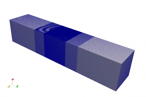
The use of porous formulation allows to employ a structured mesh, composed by only hexahedral elements. In the region where the matrix is placed, the grid is refined, in order to guarantee a good accuracy in the reproduction of the geometry under investigation. The choice of the grid for all the simulations is done after a mesh independence analysis, whose results are shown in Table 3. The pressure drop through the domain is evaluated, and the relative difference between the results for each mesh level and the previous level is also reported. It is possible to notice that the mesh composed by 2,025,000 cells leads to results that are considered mesh-independent, with a difference lower than 1%. Such a mesh is shown in Figure 3.
Table 3. Mesh independence results
|
# cells |
Δp [Pa] |
Difference |
|
254700 |
2377.08 |
|
|
600000 |
2890.50 |
17.76 % |
|
2025000 |
3183.31 |
9.20 % |
|
4800000 |
3215 |
0.99 % |
Figure 3. Structured mesh used for the computations
2.4 Boundary conditions
As regards boundary conditions, a uniform velocity profile along the inlet section is imposed, whereas a fixed pressure on the outlet section (i.e. the atmospheric pressure) is set.
In this work, the operating conditions of the engine regenerator corresponds to the heat transfer from the hot stream to the wires. Indeed, the wires are kept at a fixed temperature (Twall=300K) lower than the inlet fluid temperature (Tin=500K).
In order to reproduce the working phase of the regenerator, some conditions need to be forced in the model. Specifically, the solver is modified in order to impose the velocity equal to 0 and the temperature to a value of 300 K in the cells that correspond to the wires.
In this work, several velocity values at the inlet section are considered, as summarized in Table 4, where also the corresponding Reynolds numbers are reported, computed by the formula:
$\operatorname{Re}=\frac{\rho {{v}_{\max }}{{d}_{h}}}{\mu }$
where ${v}_{\max}=v_{in}/\pi_v$ and μ is the kinematic viscosity of the fluid.
Table 4. Summary of the flow conditions studied
|
Re |
7.84 |
24.61 |
60.11 |
92.08 |
141.46 |
185.6 |
|
uin [m/s] |
0.64 |
2.00 |
4.88 |
7.49 |
11.5 |
15.09 |
The results are given in terms of friction coefficient, in order to represent the pressure losses, and of average temperature at the outlet section, as regards the thermal performances. The friction coefficient is computed as:
${{c}_{f}}=\frac{\Delta p}{\frac{1}{2}\rho v_{\max }^{2}}$, where $\Delta p=p_{out}-p_{in}$
The outlet temperature is normalized w.r.t. the difference between inlet and wires temperature, by considering:
$\phi \text{=}\frac{{{T}_{out}}-{{T}_{in}}}{{{T}_{wires}}-{{T}_{in}}}$ (10)
For the thermal performance definition, the average temperature on the outlet section area is employed. The outlet temperature gives a measure of the total heat transferred to wires in the domain. Hence, it is a good choice to compute the thermal efficiency of the regenerator. Indeed, a higher difference between the inlet temperature and the outlet temperature corresponds to a higher efficiency of the regenerator itself. By considering Eq. 10, values of ϕ close to unit corresponds to higher efficiencies.
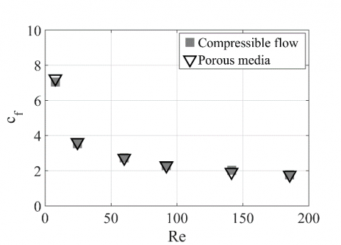
In Figure 4 the friction coefficient is plotted versus the Reynolds number. The results obtained by means of the porous media model are compared with those obtained in [7]. It is possible to observe a good agreement between the two curves, characterized by the same trend. By comparing the results corresponding to the same Re, the maximum difference obtained is of about 5 %.
Figure 4. Friction coefficient as a function of Re for compressible flow and porous model, Tin=500 K and Twall=300 K
As already predicted, the trend of the friction coefficient is always decreasing, because the compressibility effects are negligible.
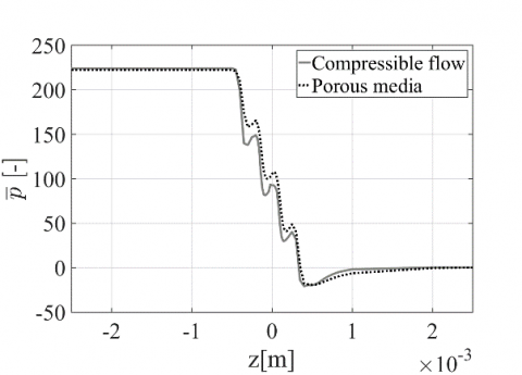
In Figure 5, the dimensionless pressure profiles along the centerline versus z coordinate, obtained with the two models, are compared by considering the case with Re=92. It is possible to observe that the two profiles have a very similar shape. In correspondence of the wires, sudden pressure drops are observed with both models. The highest decrease of pressure occurs through the first row of wires with the compressible flow model, whereas the drop observed by considering the porous model is smaller, due to the absence of interface between wires and flow. Besides, by observing the velocity fields, normalized w.r.t. the maximum velocity (Figure 6), some differences can be appreciated. Indeed, the absence of interface is leading to lower values in correspondence of the first row of wires, which is strictly related to the lower pressure drop. However, by considering the third row of wires, a higher velocity is observed in the porous model, which provides the total pressure drop through the matrix expected from the simulation. Hence, the use of the Darcy term in the momentum equation enables to predict the same value of the friction coefficient as in the standard CFD simulation.
As regards the temperature distribution, Figure 7 shows ϕ profile as a function of the Reynolds number. The standard simulations and the porous media model give similar results, with a maximum difference of 2 %. The figure shows that ϕ decreases by increasing Reynolds number, since a progressive reduction of the thermal efficiency of the system occurs by increasing Re.
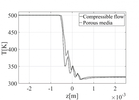
The temperature profiles along the centerline of the domain, obtained by using the porous model and a classical CFD computation, are reported in Figure 8 in the case Re=92. They are characterized by four drops of the fluid temperature, due to the presence of the wires. Although the fluctuations of temperature values are located in the same positions in the two cases, the amplitude of the temperature oscillations are different by using the two different models. This is related to the absence of the interface between solid and fluid zone in the case the porous media is used. However, the results are globally corrected by means of the heat source introduced in the regenerator region, as explained in Section 2.
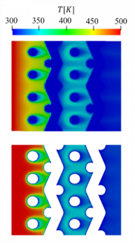
In Figure 9 the temperature fields around the wires obtained with the two models are compared, thus observing in correspondence of the first line of wires a lower temperature in the porous model w.r.t. the one with solid walls.
Figure 5. Dimensionless pressure profile along z-direction, Tin=500 K and Twall=300 K– Re=92
Figure 6. Normalized velocity contour plots on YZ middle plane of the wires matrix, Tin=500 K and Twall=300 K– Re=92
Figure 7. Dimensionless outlet temperature as a function of Re for compressible flow and porous model, Tin=500 K and Twall=300 K
Figure 8. Temperature profiles along z-direction, Tin=500 K and Twall=300 K– Re=92
The difference is due to the presence of the heat source in the region where the regenerator is placed. However, the porous model allows to correctly describe the global performance of the regenerator.
After checking the accuracy of the porous model as defined in this work, some considerations are useful with reference to the computational cost of such simulations. The use of a porous media enables to perform a simulation in a computational time that is more than ten times lower than that of a standard CFD simulation which employs the actual regenerator geometry. However, the number of computational cells in the standard CFD simulations is lower than that used with the porous media (1,523,969 vs 2,025,000 cells). Nevertheless, the same level of convergency is obtained in about 800 iterations with the porous model, whereas about 10,000 iterations are required with the other simulation.
Figure 9. Temperature contour plots on YZ middle plane of the wires matrix, Tin=500 K and Twall=300 K– Re=92
An analysis of the Stirling engine regenerator performances represents a crucial point in the study of such kind of engine. This work aims to define a numerical model able to describe both the global performance parameters, i.e. friction coefficient and thermal efficiency, and the behavior of the fluid flowing through the regenerator by using a novel numerical approach based on the porous media approximation. Instead of considering the regenerator wires as walls or as a unique block of porous material, the geometry of the wires has been defined by considering fully solid zones, whereas the flow is considered as a fully fluid zone. In order to reproduce the presence of an interface between wires and flow, an artificial boundary layer, for correcting the aerodynamic performance, and a heat source in the domain, for describing the heat transfer between regenerator and air, have been introduced. Besides, the Darcy term is added in the momentum equation and the thermal properties are defined by using a linear interpolation between the fluid and the solid material properties.
The regenerator has been studied under laminar conditions and by assuming the flow as incompressible. The results show that the model allows to achieve a good agreement with a standard CFD model in terms of both friction coefficient and spatially-averaged temperature at the outlet section. On the other hand, slight discrepancies are observed in terms of velocity distribution due to the absence of a geometrical interface. Specifically, with the same total pressure drop, some pressure differences are locally found. A similar behavior is also observed for the temperature profiles. However, the heat source contribution provides good global performance of the Stirling component.
Finally, the model gives accurate global performances of the regenerator though some differences are observed in the fluid velocity and temperature distributions. Moreover, the use of the proposed model allows a considerable reduction of the total computational cost of the simulations.
|
c |
specific heat, J. kg-1. K-1 |
|
k |
thermal conductivity, W.m-1. K-1 |
|
Greek symbols |
|
|
ε |
Fluid volume fraction |
|
f |
Dimensionless outlet temperature |
|
ρ |
Density, kg.m-3 |
|
µ |
dynamic viscosity, kg. m-1.s-1 |
|
Subscripts |
|
|
m |
mixture |
|
f |
fluid |
|
s |
solid |
[1] Andersen SK, Carlsen H, Thomsen PG. (2006). Numerical study on optimal Stirling engine regenerator matrix designs taking into account the effects of matrix temperature oscillations. Energy Conversion and Management 47: 894-908. https://doi.org/10.1016/j.enconman.2005.06.006
[2] Tanaka M, Yamashita I, Chisaka F. (1990). Flow and heat transfer characteristics of the Stirling engine regenerator in an oscillating flow. JSME International Journal. Ser. 2, Fluids Engineering, Heat Transfer, Power, Combustion, Thermophysical Properties 33: 283-289. https://doi.org/10.1299/jsmeb1988.33.2_283
[3] Gheith R, Hachem H, Aloui F, Nasrallah SB. (2015). Experimental and theoretical investigation of Stirling engine heater: Parametrical optimization. Energy Conversion and Management 105: 285-293. https://doi.org/10.1016/j.enconman.2015.07.063
[4] Costa SC, Tutar M, Barreno I, Esnaola JA, Barrutia H, Garcı́a D, González MA, Prieto JI. (2014). Experimental and numerical flow investigation of Stirling engine regenerator. Energy 72: 800-812. https://doi.org/10.1016/j.energy.2014.06.002
[5] Costa SC, Barrutia H, Esnaola JA, Tutar M. (2014). Numerical study of the heat transfer in wound woven wire matrix of a Stirling regenerator. Energy Conversion and Management 79: 255-264. https://doi.org/10.1016/j.enconman.2013.11.055
[6] Barreno I, Costa SC, Cordon M, Tutar M, Urrutibeascoa I, Gomez X, Castillo G. (2015). Numerical correlation for the pressure drop in Stirling engine heat exchangers. International Journal of Thermal Sciences 97: 68-81. https://doi.org/10.1016/j.ijthermalsci.2015.06.014
[7] Faruoli M, Viggiano A, Magi V. (2018). An investigation of thermo-fluid dynamic performance of a Stirling engine regenerator by means of OpenFOAM. Modelling, Measurement and Control B 87: 151-158. https://doi.org/10.18280/mmc_b.870306
[8] Bello F, Viggiano A, Fanelli E, Magi V. (2014). A CFD analysis of the air flow through the matrix regenerator of Stirling engines. in ISEC Conference Proceedings.
[9] Buonomo B, Pasqua ADI, Ercole D, Manca O. (2018). Porosity effect on thermal and fluid dynamic behaviors of a compact heat exchanger in aluminum foam. Revue des Composites et des Matériaux Avancés 28: 305-322. https://doi.org/10.1088/1742-6596/745/3/032141
[10] Costa SC, Barreno I, Tutar M, Esnaola JA, Barrutia H. (2015). The thermal non-equilibrium porous media modelling for CFD study of woven wire matrix of a Stirling regenerator. Energy Conversion and Management 89: 473-483. https://doi.org/10.1016/j.enconman.2014.10.019
[11] Mahkamov K. (2006). Design improvements to a biomass Stirling engine using mathematical analysis and 3D CFD modeling. Journal of Energy Resources Technology 128: 203. https://doi.org/10.1115/1.2213273
[12] Othmer C. (2008). A continuous adjoint formulation for the computation of topological and surface sensitivities of ducted flows. International Journal for Numerical Methods in Fluids 58: 861-877. https://doi.org/10.1002/fld.1770
[13] Borrvall T, Petersson J. (2002). Topology optimization of fluids in Stokes flow. International Journal for Numerical Methods in Fluids 41: 77-107. https://doi.org/10.1002/fld.426
[14] Nield DA, Bejan A. (2013). Convection in porous media. 4th ed New York: Springer Science+Business Media.
[15] Ushakov PA. (1979). Problems of heat transfer in cores of fast breeder reactor, heat transfer and hydrodynamics of single-phase flow in rod bundles. Izd. Nauka.