OPEN ACCESS
A Loss of Coolant Accident (called ICE cat. IV) is postulated to occur in the ITER Vacuum Vessel due to a rupture of a shielding blanket cooling piping. The mitigation of this accident is realized by means of a Pressure Suppression System, constituted by 4 Tanks of 100 m3 of volume each.
The Pressure Suppression Tanks (PSTs) system operates at sub-atmospheric pressure. No experimental results of steam condensation at sub atmospheric pressure conditions have been found in the technical literature.
Therefore, both analytical-numerical analyses and experimental tests were carried out at the University of Pisa on a 1:22 scale apparatus, simulating the PST.
Scaling studies were performed in order to calculate the effectiveness and functional performance of PST, simulating in the reduced scale apparatus the transient of steam mass flow rate occurring during the ICE IV event. The accidental scenarios have been determined considering the results of previous thermal hydraulic studies performed at ITER. Subsequently, a quite extensive experimental campaign has been carried out on the reduced scale apparatus in order to study the influence of the main thermal hydraulic parameters that characterize the steam condensation efficiency in sub-atmospheric conditions.
This paper illustrates the results of analytical and numerical analyses simulating the PST behaviour during the transient of steam mass flow rate due to the Ingress of Coolant Event. The transient has been simulated experimentally applying the elaborated scale laws. The designed tanks of the PST have matched the safety goal to reduce the system pressurization condensing the injected steam at sub-atmospheric pressure.
nuclear fusion reactor, ITER, direct steam condensation, CFD
The Loss of Coolant Accident (LOCA) scenario is one of the most challenging accident sequence for the ITER safety because it may lead to a pressurization of the Vacuum Vessel (VV) due to the sudden formation of steam and non-condensable gases (Hydrogen and Oxygen) [1-3]. In such an event, the steam is discharged at a high or low rate, according to the postulated event conditions [4-6], into the Vacuum Vessel Pressure Suppression System (VVPSS).
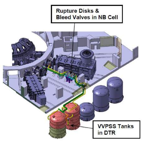
The VVPSS is located in the Drain Tank Room (DTR), as shown in Figure 1. The VVPSS is designed to protect the VV from over pressurization caused by accidental conditions. It is made of four vapour suppression tanks (VSTs) (see Figure 2). In particular, an Inlet Coolant Event (ICE) is assumed as an accidental scenario.
VVPSS behaves, in principle, similarly to a containment of boiling water reactor even if it differentiates because it operates at sub-atmospheric pressure [1, 4, 7-8]. This peculiarity makes innovative and almost unique this investigation of the steam direct condensation at sub-atmospheric pressure.
The main components of VVPSS are the four Vapor Suppression Tanks (VSTs) having a height of 4.7 m, diameter of 6.3 m and overall inner volume of 100 m3 each. They are partially filled with water in order to condense directly the steam and thus to dump the pressure. Each tank contains a single vertical sparger tube to discharge the steam and the non-condensable gases.
Figure 1. Location of the four VSTs in the tokamak cooling water system
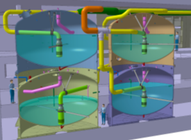
The design configuration for the VSTs is shown in Figure 2. One tank, Small LOCA Tank (SLT), is used to manage small LOCAs and Loss of Vacuum Accidents (LOVAs). This tank contains 40 m3 of water. The other three Tanks, Large LOCA Tanks (LLTs), contains 60 m3 of water and are used to manage higher category events.
Figure 2. Configuration of VSTs (3 LLT and 1 SLT)
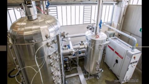
As previously mentioned, the VVPSS needs of experimental assessment since tests at its operating conditions are not available in the technical literature. Therefore, a research program with a “small-scale” experimental rig (about 1:22 reduced scale) has been carried out at DICI-University of Pisa, performing about 400 tests.
The experimental facility with its main components is shown in Figure 3. A more detailed description of the facility is given in [1-2]. The steam is injected inside the condensation tank through a removable single or multiple-holed (with 1 to 18 holes) sparger system.
With the ‘small scale’ experimental rig the main steam condensation regimes have been deeply investigated. A ‘Large Scale’ experimental rig (geometrical scale 1/1.08 and steam mass flow rate scale 1/10) is under construction at the University of Pisa, whose 3D rendering is shown in Figure 4. The main components are the Experimental Test Tank (ETT) of 92 m3 of volume and the electric steam generator of 1.5 MWe of power.
2.1 Similitude analysis
A similitude analysis has been elaborated and the scaling laws have been applied for simulating accidental scenarios which could occur in the Vacuum Vessel of ITER.
Obviously, the main parameter of steam direct condensation is the volume of the tank and the quantity of water contained in it.
Figure 3. Reduced scale experimental rig (1/22 scale)
Figure 4. Large scale experimental rig (1/1.08 scale)
From the experimental tests, we have deduced that the condensation regimes depend mainly on:
The selected geometric scaling factor (S) is dependent on the ratio between the actual volume of the condensation tank (Vact) and the volume of the scaled tank (Vscal), that is S = Vact/Vscal.
Furthermore, the ratio between water volume to vacuum volume has to be equal to S in order to have the same physical mechanism of steam direct condensation in full scale and in the reduced scale condensation tank.
The steam mass flow rate per hole, downstream pressure (in front of the hole) and water temperature have to be the same in the full-scale and reduced scale tank.
Since in the real transient conditions, the steam condensation has a relatively slow dynamic process evolution, it can be considered a sequence of steady state conditions and, in consideration of that, the time dependency could be neglected at first approximation. Thus, we can obtain similar condensation regimes, in the full-scale as well as in the reduced scale system, if:
At scaled time, the average water temperature, Tw, and the pressure, Pw, are the same in the full-scale as well as in the reduced scale system.
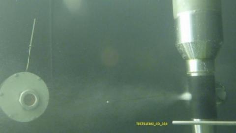
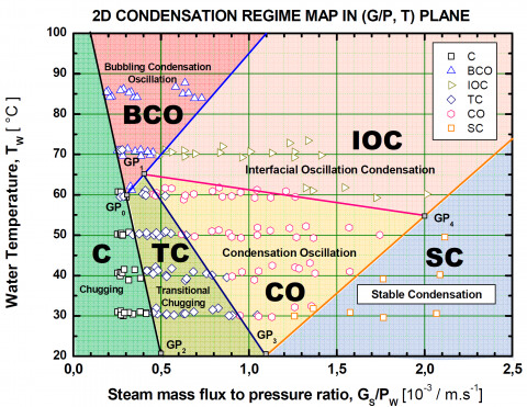
The experimental tests have permitted to identify six main condensation regimes (CR) (based on the video recorded during the tests) which are the following:
(a) SC: Tw=30 °C; Pw=30 kPa; Hw=1 m; qs=5 g/s
(b) OC: Tw=50 °C; Pw=60 kPa; Hw=1 m; qs=5 g/s
(c) IC: Tw=70 °C; Pw=40 kPa; Hw=1 m; qs=5g/s
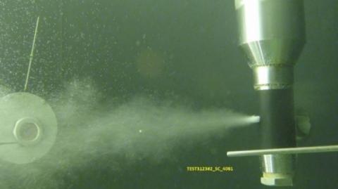
Figure 5. CRs: Stable Condensation (SC), Oscillation Condensation (OC) and Interfacial Oscillation (IO)
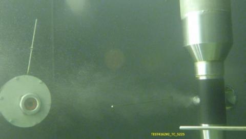
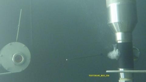
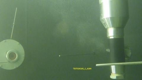
Figures 5 and 6 illustrate the shape of the steam jet obtained in the experimental tests at the different conditions. The experimental results of the water average temperature, Tw and of the downstream pressure Pw, permitted to determine a CR map (Figure 7), which defines the condensation zones in terms of the water average temperature versus the Gs/Pw ratio [4].
The stable condensation at sub-atmospheric pressure is reached for a steam mass flow rate per unit of area, Gs, about ten times smaller than that correspondent at atmospheric pressure.
(d) TC: Tw=40 °C; Pw=70 kPa; Hw=1 m; qs=2.5 g/s
(e) BCO: Tw=40 °C; Pw=70 kPa; Hw=1 m; qs=2.5 g/s
(f) C: Tw=30 °C; Pw=80 kPa; Hw=2 m; qs=1.5 g/s
Figure 6. Condensation regimes: Transitional Chugging (TC), Bubbling Oscillation Condensation (BOC) and Chugging (C)
Figure 7. Experimental condensation regimes map
ANSYS FLUENT code [10] was used for investigating the two different steam Direct Contact Condensation (DCC) transient scenarios (A and B) at sub-atmospheric conditions.
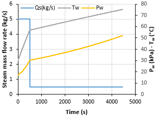
The trend of LOCA accident (ICE cat. IV) is plotted in Figure 8. The maximum steam mass flow rate managed in each LLT is about 4 kg/s. The performed CFD simulations aim to verify the behavior of the ‘Large Scale’ tank at the maximum steam flux (that is in Stable Condensation regime) and at the minimum one (in the Chugging regime).
Figure 8. Steam mass flow rate versus time produced by the ICE Cat. IV event
The peak of mass flow rate is maximized at a constant value of 5 kg/s for a transient of 500 s, while the minimum value is fixed at 0.5 kg/s for about 3000 s.
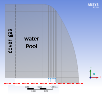
The transients have been simulated for both the ITER-LLT and the ETT and the CFD analyses were carried out also in order to assess the elaborated scaling laws. In both these analyses, FLUENT 2D axisymmetric model was selected for reducing calculation time. In order to simulate water liquid pool and cover gas domains, the multiphase model Volume of Fluid (VOF) was adopted.
The latent heat released during the steam condensation was simulated by means of energy source (W/m3) positioned in front of the injection holes (condensation region). To take into account buoyancy phenomena in the liquid phase, a liquid density function of temperature between 0 and 98 °C was implemented.
The first scenario (A) was characterized by high superheated steam mass flow rate, 5 kg/s, at 130 °C injected horizontally into saturated water pool at 30 °C, through 1000 holes of 10 mm of diameter, arranged on 20 circumferential levels with 50 holes each (first row at a depth of about 1.3 m).
FLUENT models of both LLT (100 m3) and ETT (92 m3) geometrical configurations are shown in Figure 9 and 10, respectively.
Red dashed-dot line is the vertical axis of symmetry of the tank and the five light blue arrows highlights the corresponding five circumferential openings having the equivalent flowing area of 1000 holes.
In the second analysed scenario (B), about 0.5 kg/s of steam at 130 °C was condensed into the ETT saturated water pool at 50 °C. Two numerical models B.1, B.2 were developed which differ for the simulation of the energy zone, that is, the area of the model where it is assumed that the latent heat of condensation is released:
- Model B.1, 1000 holes merged in five openings of equal area; the heat source is released in 5 annular zones having 10.94 mm of height and radial width of L= 10 mm.
- Model B.2, 100 holes merged in one injection opening with a close annular heat source having 5.47 mm of height and radial width of L=10 mm.
The upper part of ETT (top head beyond the dashed line) was not simulated in order to reduce calculation time.
The two different boundary conditions of the models B considered that a steam mass flow rate of 0.5 kg/s is distributed uniformly on 1000 holes determining a Chugging regime. This is the assumption of model B.1.
Figure 9. FLUENT model of ITER LLT
Figure 10. FLUENT model of ETT
Actually we can assume that the steam is discharged only by a reduced number of holes which can be estimated on the basis of critical mass flow rate.
The critical flowing area at steam working conditions corresponds to about the upper 90 holes (i.e. about the first two upper rows of 50 holes each). In these conditions, the longitudinal extension of steam jet plume is equal to 92 mm. This value is consistent with an empirical correlation as function of downstream pressure, mass flow rate and water pool temperature [9].
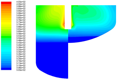
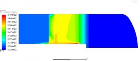
Figure 11 illustrates the distribution of temperature in the LLT and in the ETT at time instants determined through the scaling laws. Figure 12 shows the ETT temperature distribution for 0.5 kg/s steam released; it accounts for the effects due to the slight different amount of water of the two models.
Figure 11. Contour plot of temperature [K] at 440 s for ETT and at 500 s for LLT
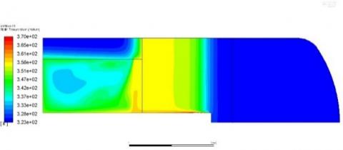
(a) Energy zone L=10 mm a t=1808 s
(b) Energy zone L=92 mm a t=1842 s
Figure 12. Contour plot of temperature [K] at t=1842 s for the model B.1 (a) and model B.2 (b)
In all the simulations, the hot water moves along the sparger reaching the water free surface and after it expands radially and axially towards the bottom. A smaller radial average temperature is obtained for the ITER LLT due to its greater radius. Otherwise, the axial depth of hot water is greater for the ETT. The area, where the condensation energy is released, has small influence on the temperature field.
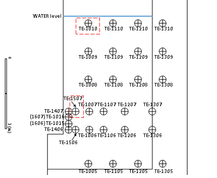
Figure 13 shows the monitor points (therein indicated with crossed circles plus TE label with a numerical identification), whose positioning was coherently defined with the ETT instrumentation layout (sensors positioning).
In the following two points are taken as reference for calculating the temperature time trends: TE-1010 close to the water free level at inner radial position and TE-1507 in front of the injection region.
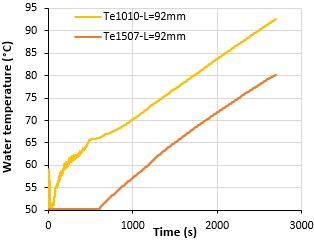
The correspondent temperature diagrams for the two models B are shown in Figure 14 and 15, respectively.
The main difference of the results obtained from the two models is the greater axial temperature difference in the model B2 (about 15 °C) which is constant in almost all the transient. The temperature difference for the model B2 changes during the transient reaching the value of about 5 °C at the end.
Figure 13. Monitor points positioning for temperature time trends calculations
Figure 14. Temperature trends at reference points for the model B1
Figure 15. Temperature trends at reference points for the model B2
During the experimental tests, superheated steam (at Ts=130 °C and at Ps ranging between 30-150 kPa) is discharged into water by means of the sparger. It transfers continuously energy to the water at low temperature and it cools down until it achieves the saturation temperature corresponding to the local pressure condition in order to condense.
When the steam condenses, it changes its thermodynamic phase from gas to liquid (hot water), by releasing latent heat to water, and it continues to transfer heat to the water until the thermal equilibrium is reached. As a result, the water is heated up. Therefore, the measurement of the mean water temperature before and after steam discharge, DTw, allows to determine the condensation rate and, thus, enables to assess the efficiency of the condensation process at the prevailed conditions.
In the performed tests, at any instant of time, the mean temperature of water in the condensation tank was determined through the measurements provided by temperature sensors located within the water.
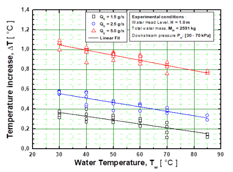
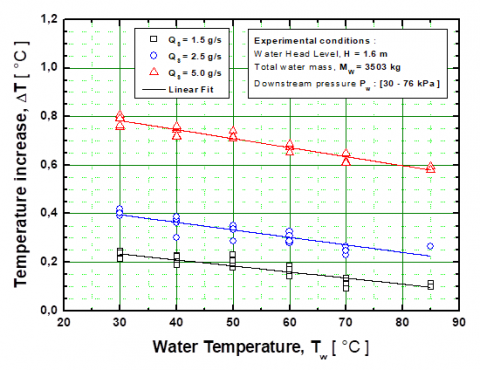
Figure 16 and 17 represent the behaviour of the average water temperature increase as a function of the initial water temperature of the tank in the range 30 ÷ 85 °C, for different steam mass flow rates (Qs=1.5, 2.5, 5 g/s) and water head levels at the sparger hole, Hw=1.0 m and Hw=1.6 m, respectively.
The downstream pressure values in front of the sparger hole, Pw, ranges from 30 kPa to 76 kPa.
Figure 16. Water temperature increase as a function of the initial water temperature (Qs=1.5, 2.5, 5 g/s; H=1 m; Pw = 30÷ 70 kPa)
Figure 17. Water temperature increase as a function of the initial water temperature (Qs=1.5, 2.5, 5 g/s; H=1.6 m; Pw = 30 ÷ 76 kPa)
Figure 18 shows the water temperature increase at atmospheric pressure.
The previous figures show that the water temperature increase (DTw) is independent from the downstream pressure. DTw can be considered proportional to the total steam mass discharged (MS) and inversely proportional to the total mass of water in the tank (MW). The proportionality constant q(Tw), that we can call effective thermal capacity, depends only on the water temperature. Assuming total condensation in water, DTw can be written as:
$\Delta {{T}_{W}}=\theta ({{T}_{W}})\,\frac{{{M}_{S}}}{{{M}_{W}}}$ (1)
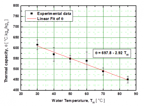
We have determined experimentally the values of the effective thermal capacity q(Tw) for initial water temperature in the range 30 ÷ 85 °C (Figure 19). The experimental data have been fitted linearly by the regression:
$\theta ({{T}_{W}})\,=697.8-2.92\,\,{{T}_{W}}$ (2)
Figure 18. Water temperature increase ΔTw at atmospheric pressure as function of the water temperature (Qs=2.5g/s- Hw=1 m; Pw = 111 kPa; Qs=12. g/s-Hw=1.6 m- Pw = 117 kPa)
Figure 19. Experimental data of effective thermal capacity of water (q) as a function of the water temperature
On the basis of the Eq. (1) and (2) and of the similitude laws, described in paragraph 2.1, any accidental scenarios can be simulated analytically in the full scale or reduced scale tank, obtaining the average water temperature, Tw, and the downstream pressure Pw versus time. These values permit to determine the evolution of the scenario in the map of the condensation regimes. In particular, Tw is calculated by means of the steam mass discharged in the tank, Ms, and the total mass of the water, Mw using Eq. (2).
After the calculation of Tw, the downstream pressure Pw is given by the (3):
$Pw=\,{{P}_{FSV}}+{{\rho }_{w}}({{T}_{w}})\,g\,{{H}_{w}}$ (3)
where PFSV, rw are the steam saturation pressure and the water density at the temperature Tw. PFSV is assumed to be the pressure in the vacuum space of the tank and it is given by the following equation:
$P_{FSV}=P_{sat}=c_1[1-c_2 θ(1-c_3 θ+c_4 θ^2-c_5 θ^3)]$ (4)
being q=Tw/100 and c1=0.97417; c2=1.13943; c3=38.919; c4=36.036; c5=88.345.
The correlation (4) is valid in the range 10°C≤Tw≤110°C.
The water density versus temperature is given by the following correlation:
$ρ_w=10^3(1-\frac{(T_W+288.941)(T_W-3.9863)^2}{5.089292*10^5(T_W+68.12693)})$ (5)
rw(Tw) is given in kg/m3 and the correlation is valid in the range 10 °C≤TW≤100 °C.
Figure 20 illustrates the results of the analytical model applied at the ETT considering the transients simulated by the CFD. Once the Pw and Tw have been obtained it is possible to determine the condensation regimes calculating the unit steam mass flow rate to downstream pressure Pw ratio, by means of the following equation:
${{\left( \frac{{{G}_{S}}}{{{P}_{W}}}\ \right)}_{hole}}=\,\left( \frac{{{q}_{s}}}{{{A}_{h}}\,{{P}_{W}}} \right)$ (6)
Figure 20. Application of the analytical model at ETT
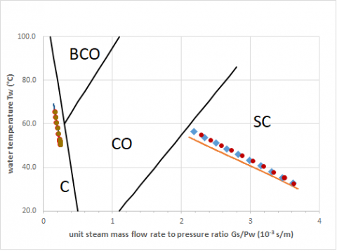
The steam mass flow rate Qs=5 kg/s in a sparger of 1000 holes of 10 mm of diameter determines points of coordinates (Gs/Pw, Tw) which are localized in the stable condensation zone. While the points correspondent to Qs=0.5 kg/s are localized in the chugging zone.
The curves of the condensation regimes are illustrated in Figure 21 as coloured solid lines. The black lines subdivide the space in areas of different CRs.
Figure 21 compares the results of the CFD simulations and those of the analytical model in the condensation regime map. The solid lines refer to the analytical results while the symbols refer at the CFD results correspondent at different instants of time of the transients.
In the stable condensation zone CFD results for the full scale (diamonds) and the reduced scale ETT (circles) are compared with the analytical results. In the chugging zone, the analytic results are compared only with the results of CFD simulations of ETT (model B.1 and B.2).
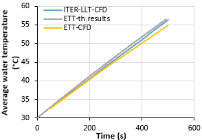
Applying the scale laws (that in this case corresponds to an amplification with the factor 1/S of the time of the reduced scale), results in term of water average temperature versus time are illustrated in Figure 22.
The obtained values are almost coincident in the first part of transient. The scaled results of the reduced scale condensation tank are 1 °C smaller than the other at the end of the greatest steam mass flow rate transient. This small discrepancy is due essentially to the different D/H (Diameter/Height) ratio of the full scale and reduce scale tanks. This different D/H ratio determines a different temperature difference along the height of the tanks.
-Diamonds: full scale tank – Circles: reduced scale ETT
Figure 21. Map of condensation regimes: comparison between analytical and numerical results
Figure 22. Average water temperatures vs time obtained by the CFD simulations and analytical results
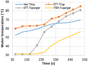
Figure 23. Water average temperatures versus time at different heights of the full scale tank (ITER) and reduced scale tank (ETT)
Figure 23 illustrates the water average temperatures at two heights of the tanks: at the free water surface (Ttop) and at the sparger holes (Tsparger). The average value is calculated for a radial distance of 2 m (equal to the ETT radius). Figure 23 shows that at the end of transient, the temperature difference is equal to about 4 °C for ETT while it is about 15° C for the ITER tank.
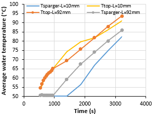
The influence of the length of steam jet on the axial difference of temperature is shown in Figure 24. A greater length of steam jet produces a smaller axial difference of temperature (about 8 °C) which remains almost constant in all the transients. A shorter length of steam jet produces a greater axial difference of temperature although at the end of transient the temperature difference is almost equal.
Figure 24. Water average temperatures vs time at different heights of the reduced scale tank (ETT) (different lengths of steam jet: L=10mm-L=92mm)
This paper illustrates the results of experimental tests, analytical model and CDF simulations concerning the steam direct condensation in water at sub-atmospheric pressure.
The tests have been performed in a reduced scale experimental rig simulating the ITER safety system called VVPSS. A similitude analysis has been developed in order to extrapolate the results obtained with the reduced scale experimental rig to the full scale system.
The CFD analyses permitted to assess the scale laws and demonstrate the capability of a large-scale condensation tank to simulate very well the physical phenomena which occur in the actual full scale Vapor Suppression Tank even if the Diameter/Height ratio is different. This different D/H ratio determines a different temperature difference along the height of the tanks.
The heat transfer occurs preferably in the axial direction in the longer ETT and in radial direction in the ITER tank. All the water, in both the tanks, is involved in the condensation process. Therefore, the water average temperature and the downstream pressure (in front of the sparger holes) are equal, resulting in the same condensation regimes.
The analytical model, developed based on the experimental results, seemed to describe well the global process of steam condensation at sub-atmospheric pressure. In addition, it permitted to determine the different condensation regimes depending on the transient of the steam mass flow rate due to accidental events and the water average temperature and downstream pressure in the condensation tank.
The views and opinions expressed herein do not necessarily reflect those of the ITER Organization.
[1] Mazed D, Lo Frano R, Aquaro D, Del Serra D, Sekachev I, Olcese M. (2018). Experimental investigation of steam condensation in water tank at sub-atmospheric pressure. Nuclear Engineering and Design 335(15): 241-254. https://doi.org/10.1016/j.nucengdes.2018.05.025
[2] Mazed D, Lo Frano R, Aquaro D, Del Serra D, Sekachev I, Orlandi F. (2016). Experimental study of steam pressure suppression by condensation in a water tank at sub-atmospheric pressure. Proceedings ICONE24, Charlotte, North Carolina (USA), pp. V002T06A003. https://doi.org/10.1115/ICONE24-60029
[3] Lo Frano R, Mazed D, Aquaro D, Del Serra D, Sekachev I, Giambartolomei G. (2017). Methodology to investigate vibration phenomena caused by the steam condensation at sub-atmospheric condition. Proceedings of 25th International Conference on Nuclear Engineering, Shanghai (China), pp. V005T05A042. https://doi.org/10.1115/ICONE25-67448
[4] Lo Frano R, Mazed D, Aquaro D, Del Serra D, Orlandi F. (2017). Experimental investigation of functional performance of a vacuum vessel pressure suppression system of ITER. Fusion Engineering and Design 122: 42-46. https://doi.org/10.1016/j.fusengdes.2017.09.010
[5] Lo Frano R, Mazed D, Olcese M, Aquaro D, Del Serra D, Sekachev I, Giambartolomei G. (2018). Investigation of vibrations caused by the steam condensation at sub-atmospheric condition in VVPSS. Fusion Engineering and Design 136(B): 1433-1437. https://doi.org/10.1016/j.fusengdes.2018.05.031
[6] Lo Frano R, Aquaro D, Olivi N. (2016). Fluid dynamics analysis of loss of vacuum accident of ITER cryostat. Fusion Engineering and Design 109-111(B): 1302–1307. https://doi.org/10.1016/j.fusengdes.2015.12.038
[7] Shibata M, Takase K, Watanabe H, Akimoto H. (2002). Experimental results of functional performance of a vacuum vessel pressure suppression system in ITER. Fusion Engineering and Design 63-64: 217-222. https://doi.org/10.1016/S0920-3796(02)00242-9
[8] Takase K, Ose Y, Kunugi T. (2002). Numerical study on direct-contact condensation of vapor in cold water. Fusion Engineering and Design 63-64: 421-428. https://doi.org/10.1016/S0920-3796(02)00269-7
[9] Aquaro D. (2015). Experimental study of steam pressure suppression by condensation in a water tank at sub-atmospheric pressure. FDR Meeting, Cadarache, France.
[10] ANSYS FLUENT rel.19.2 – 2018 Ansys©Inc