OPEN ACCESS
The subject dealt with is an accurate semi-analytical modeling of two-dimensional radiative heat transfer. The semi-transparent medium is gray and has an absorbing-emitting rectangular shape hollowed by internal square fluid cavity, bounded by black surfaces.
The aim is to establish some benchmark results either for radiative intensity, or flux and temperature field, from which forwards analysis will be compared. Hence, analytical incoming radiative intensity, flux and temperature fields inside the gray medium are established, in function of the center coordinates of the fluid cavity. Only radiative transfer mode is considered at equilibrium state. Therefore, radiative quantities are spatially and angularly integrated using special functions in order to avoid ray effects on results. Thanks to double Gauss quadrature, which will allow to obtain numerically the radiative equations.
Finally, results validation is done when the size of internal hollowed cavity becomes very small and expected results remain with good agreement with literature.
radiative heat transfer, semi-transparent, semi-analytical
Prediction of radiative heat transfer in semi-transparent media with complex geometries remains one of the major challenges of scientists nowadays [1-2]. Because it applications give rise to many industrial interests, like solar energy system [3], thermal barriers coating, float and foams, in aerospace engineering, several techniques of predictions are used. Since, this kind of energy transfer involves both conduction and radiation transfer equations [4], only radiation transfer energy is taken in consideration here. Hence, in case of the full parallelogram shape geometry, no pure exact analytical solutions are already found, but different methods are already developed using either semi-analytical or/and numerical approximations of resolution [5-7]. This lack of analytical solutions comes from the complex geometry of media concerned. However, among some approaches developed for various geometries, the most accurate used is based on Monte-Carlo [8-9], also known as ray tracing method. Although, ray effect problem was solved, solutions were optimized later by introducing a new specific analytical function [10-11], in evaluation process of radiation quantities for better estimations.
Although, it presents some advantages on analytical point of view, it carries also several difficulties on numerical implementation because ray effect is observed.
Furthermore, considering the high quadrature dependence in spatio-angular integral approximations, that yields sometime to ray-effect phenomenon on results expected, a Discrete Ordinate Method (DOM) was implemented to solve the problem, regarding it simplicity, fastlness and accuracy. In order to reduce the ray effect impact on solutions, it has also been perfomed [12], by adding a new set of particular spatial-angular Gaussian quadrature to attenuate degree of ray effect in the medium. Despite the fact DOM method was developed and used, other more accurate numerical and experimental tools have been also established, like finite and volume finite element method [13-14], used for their excellent prediction results. In the same category of finite elements, Meshless method based on Petrov-Galerkin technic was done [15-16].
This paper focus on high analytical development in order to produce accurate benchmark results in case of rectangular gray semi-transparent medium, hollowed by internal rectangular cavity containing a static fluid flow. The results will enable other methods to compare with. Until now, no exact analytical solutions have been proposed on macroscopic dimensions, despite some numerical results existing in the literature developed on microscopic aspect. The method used in this work is quite similar of the method used in [1, 5] at radiative equilibrium. Nevertheless radiation intensity, flux and temperature field are calculated for each subdomain of ray attenuation in the medium, since internal rectangular cavity behaves like obstacle for ray propagation.
Thereby, for the proposed geometry, analytical calculations of radiative intensity and flux field are done for all incoming radiation from Eastern, Northern, Western and Southern radiations, at any attenuated point in the medium.
The final results are deduced from numerical resolution of discretization form. Hence, radiation integrals are transformed by Altaç special functions [10-11] using both angular and spatial gauss quadrature. Consequently temperature field in the medium is obtained by interation process until convergence.
2.1 Geometry and governing equations
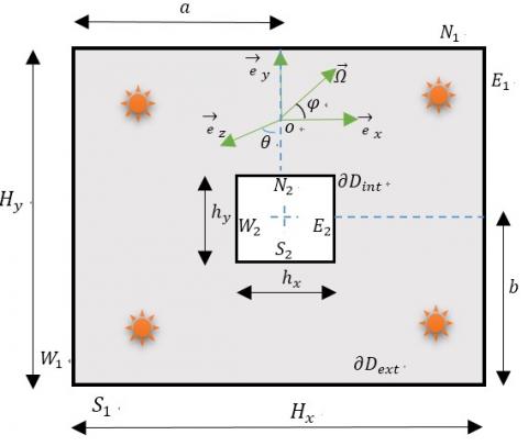
Consider a two dimensional solid /fluid semi-transparent gray medium, where, the solid matrix simultaneously emits, absorbs but does not scatter radiation, whereas the fluid, is in this study under steady state conditions. External $∂D_{ext}$ and internal $∂D_{int}$ boundary domains are at imposed temperature, and are assumed as black surfaces Figure 1. For this purpose, let ka denotes absorption coefficient, n as refractive index, where I is the radiation intensity in one direction and T as temperature field in solid medium. Therefore, only radiative heat transfer is considered as energy transfer mode at steady conditions, and given by the differential equation:
$\frac{\partial I(s,\Omega )}{\partial s}=-{{k}_{a}}I(s,\Omega )+{{n}^{2}}.{{k}_{a}}.{{I}_{b}}\left( T(s) \right)$ (1)
where, s represents the curvilinear abscissa, Ω the direction of radiation propagation inside the medium, $I_b$ the Planck’s black body radiative intensity depending of temperature medium.
Figure 1. Solid / fluid semi-transparent medium
Incident radiation at each point of the solid matrix is calculated by solving Eq. (1), which yields the result in the form:
$I(s,\Omega )={{I}_{0}}(s){{e}^{-{{k}_{a.}}\delta }}+\frac{{{n}^{2}}{{k}_{a.}}\sigma }{\pi }\int_{s=0}^{s}{{{T}^{4}}({{s}^{'}}){{e}^{-{{k}_{a.}}{{s}^{'}}}}ds}$ (2)
where, $I_0 (s)$ is radiation intensity leaving each boundary surface situated at position s, σ is the Stephan-Boltzman constant, δ is the path length followed by the ray from either external or internal boundaries to the various attenuation points in the absorbing medium.
Inside the medium, the overall radiative intensity G(s) is evaluated for all directions Ω, hence:
$G(s)=\int_{\Omega =4\pi }{I(s,\Omega )d\Omega }$ (3)
The radiative flux, is deduced from G(s) by:
${{\overrightarrow{q}}_{r}}(s)=\int_{\Omega =4\pi }{I(s,\Omega )\overrightarrow{\Omega }d\Omega }$ (4)
While temperature field is calculated from radiative flux divergence relation at radiative equilbrium state condition, playing the role of radiation source in the medium. It is done by:
$\overrightarrow{\nabla }.{{\overrightarrow{q}}_{r}}={{k}_{a}}\left( 4\pi {{n}^{2}}{{I}_{b}}\left( T(s) \right)-G(s) \right)$ (5)
2.2 Evaluation of radiative quantities
(1) Geometry of the problem
The rectangular semi–transparent medium designed with external and internal surfaces, having respectively $H_x×H_y$ and $h_x×h_y$ dimensions in (x, y) reference Figure 1. The radiation propagates though $\left( {{\overrightarrow{e}}_{x}},{{\overrightarrow{e}}_{y}} \right)$ plane and z-direction are infinite, consequently no variations over this z-axis affects any calculation. Moreover, radiation propagation is explained in terms of azimuth angle φ which represents angle yields by orthogonal projection of rays on x-axis, such 0≤φ≤2π and zenith angle θ represent deviation between z-axis and the ray, such 0≤θ≤π in this plane Figure 1. Therefore, the relation links them to direction vector $\overrightarrow{\Omega }=\left( \begin{align} & \cos \varphi \sin \theta \\ & \sin \varphi \sin \theta \\ & \cos \theta \\ \end{align} \right)$.
Neither radiative intensity, radiative flux nor temperature depends of z-axis components.
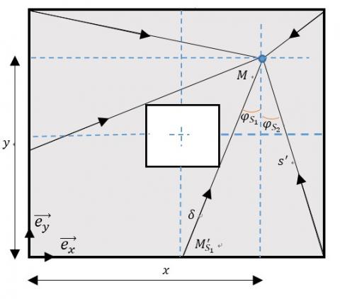
Figure 2. Attenuation of rays inside the semi-transparent medium
(2) Radiation intensity
In the present study, fluid cavity and solid semi-transparent media are located at the same center coordinate: $a=\frac{{{H}_{x}}}{2}$ and $b=\frac{{{H}_{y}}}{2}$. Hence, evaluation of radiative quantities becomes highly dependent of ratios $\frac{{{H}_{x}}}{{{h}_{x}}}$ and $\frac{{{H}_{y}}}{{{h}_{y}}}$. So, there are five positions depending of that ratios, ${{\left. \frac{H}{h} \right|}_{x,y}}<3;{{\left. \frac{H}{h} \right|}_{x,y}}=3;3<{{\left. \frac{H}{h} \right|}_{x,y}}<2+\sqrt{5};{{\left. \frac{H}{h} \right|}_{x,y}}=2+\sqrt{5}$ and ${{\left. \frac{H}{h} \right|}_{x,y}}>2+\sqrt{5}$. When a set of equations modelling the different radiative energy is calculated at one position, the other set can be deduced from the previous one.
To evaluate radiation quantities exactly from all internal and external boundary surfaces in the solid matrix, the ratio choice for this application is $\frac{{{H}_{x}}}{{{h}_{x}}}=3$, and $\frac{{{H}_{y}}}{{{h}_{y}}}=3$. The solid matrix is divided into several sub-regions, Figure 2 over which calculations are performed for each ray attenuated.
The modeling principle is shown there, only for an external southern-Est boundary surface (S1), view from ${{\varphi }_{{{S}_{1}}}}$ and carrying an imposed temperature ${{T}_{{{E}_{1}}}}$. Radiation intensity expected at attenuation point M due to absorption follows the same path length as the one coming from this point and diverges to boundary surface, due to emission of radiations in the medium [1]. Therefore, in one direction of propagation, let consider any point M' belonging to that boundary surface, the following relations are developed:
$\left\{ \begin{align} & \overrightarrow{MM}_{{{S}_{1}}}^{'}=\delta \overrightarrow{\Omega },M_{{{S}_{1}}}^{'}\in \partial {{D}_{South,1}} \\ & {{\overrightarrow{MM}}^{'}}=s'\overrightarrow{\Omega },M'\in D \\ \end{align} \right.$ (6)
where, $\delta =\frac{0-y}{\cos \varphi \sin \theta }$ and $s'=\frac{y'-y}{\sin \varphi \sin \theta }$, are respectively a ray path length from Southern boundary at temperature ${{T}_{{{S}_{1}}}}$ and from any source of radiation in the medium to the attenuation, due to absorption effect. Therefore:
$\left\{ \begin{align} & x'=x\pm (0-y)\tan \varphi ,M_{{{S}_{1}}}^{'}\in \partial {{D}_{South,1}} \\ & x'=x\pm (y'-y)\tan \varphi ,M'\in \{D\} \\ \end{align} \right.$ (7)
These previous relations in (x, y) reference coordinates are replaced inside Eq. (2). Hence, contribution of radiative intensity in one direction from this boundary becomes,
${{I}_{{{S}_{1}}}}(x,y,\theta ,\varphi )=\frac{{{\sigma }_{B}}T_{{{S}_{1}}}^{4}}{\pi }.{{e}^{-{{k}_{a}}\left\{ \frac{y}{\cos \left( \varphi -\frac{3\pi }{2} \right)\sin \theta } \right\}}}+\frac{{{k}_{a.}}\sigma }{\pi }\int_{y'=0}^{y'=y}{{{T}^{4}}(x',y')\times {{e}^{-{{k}_{a}}\left\{ \frac{y-y'}{\cos \left( \varphi -\frac{3\pi }{2} \right)\sin \theta } \right\}}}}\frac{dy'}{\cos (\frac{3\pi }{2}-\varphi )\sin \theta }$ (8)
However, radiative intensity coming from all directions belonging southern-Est surface covers the sum of angles ${{\varphi }_{{{S}_{1}}}}$ and ${{\varphi }_{{{S}_{2}}}}$, while:
${{G}_{{{S}_{1}}}}(x,y)=2\int_{\varphi =\frac{3\pi }{2}-{{\varphi }_{{{S}_{1}}}}}^{\varphi =\frac{3\pi }{2}+{{\varphi }_{{{S}_{2}}}}}{\int_{\theta =0}^{\theta =\frac{\pi }{2}}{{{I}_{{{S}_{1}}}}(x,y,\theta ,\varphi )}}\sin \theta d\theta d\varphi $ (9)
where, ${{\varphi }_{{{S}_{1}}}}={{\tan }^{-1}}\left\{ \frac{x-(a+\frac{{{h}_{x}}}{2})}{y-(b-\frac{{{h}_{y}}}{2})} \right\}$ and ${{\varphi }_{{{S}_{2}}}}={{\tan }^{-1}}\left\{ \frac{{{H}_{x}}-x}{y} \right\}$.
Firstly, let introduce one set of Bickley’s Naylor function [17], for integration of Eq.10, and given by:
${{K}_{{{i}_{n}}}}(u)=\int_{\theta =0}^{\theta =\frac{\pi }{2}}{{{e}^{-\frac{u}{\sin \theta }}}}{{\left( \sin \theta \right)}^{n-1}}d\theta ,n\in N,u\in {{R}^{+}}$ (10)
In order to transform angular integral dependence in terms of θ to spatial one, a change of variable is done, and a new relation is obtained:
${{G}_{{{S}_{1}}}}\left( x,y \right)=\frac{2{{\sigma }_{B}}T_{{{S}_{1}}}^{4}}{\pi }\int_{\varphi =0}^{\varphi =+{{\varphi }_{{{S}_{1}}}}}{{{K}_{{{i}_{2}}}}}\left( \frac{{{k}_{a}}y}{\cos \varphi } \right)d\varphi +\frac{2{{\sigma }_{B}}T_{{{S}_{1}}}^{4}}{\pi }\int_{\varphi =0}^{\varphi =+{{\varphi }_{{{S}_{2}}}}}{{{K}_{{{i}_{2}}}}}\left( \frac{{{k}_{a}}y}{\cos \varphi } \right)d\varphi +\frac{2{{k}_{a.}}{{\sigma }_{B}}}{\pi }\int_{\varphi =-{{\varphi }_{{{S}_{1}}}}}^{\varphi ={{\varphi }_{{{S}_{2}}}}}{\int_{y'=0}^{y'=y}{{{T}^{4}}}\left( x',y' \right)}\times {{K}_{{{i}_{1}}}}\left( \frac{{{k}_{a}}\left( y-y' \right)}{\cos \varphi } \right)dy'\frac{d\varphi }{\cos \varphi }$ (11)
Secondly, Altaç function [17], is used for n∈N, $u∈R^+$, given by:
${{B}_{i{{s}_{n}}}}(u,\theta )=\int_{\varphi =0}^{\varphi =\theta }{{{K}_{{{i}_{n}}}}}\left( \frac{u}{\cos \varphi } \right){{\left( \cos \varphi \right)}^{n-2}}d\varphi $ (12)
By taking in consideration the ${{K}_{{{i}_{n}}}}$ parity function, radiation intensity for all radiations coming from eastern boundary surface and attenuated by absorption process inside each point of the solid matrix is performed by:
$\begin{align} & {{G}_{{{S}_{1}}}}\left( x,y \right)=\frac{2{{\sigma }_{B}}T_{{{S}_{1}}}^{4}}{\pi }\left\{ {{B}_{i{{s}_{2}}}}\left( {{k}_{a}}y,{{\tan }^{-1}}\left\{ \frac{x-\left( a+\frac{{{h}_{x}}}{2} \right)}{y-\left( b-\frac{{{h}_{y}}}{2} \right)} \right\} \right) \right\}+\frac{2{{\sigma }_{B}}T_{{{S}_{1}}}^{4}}{\pi }\left\{ {{B}_{i{{s}_{2}}}}\left( {{k}_{a}}y,{{\tan }^{-1}}\left\{ \frac{{{H}_{x}}-x}{x} \right\} \right) \right\}\text{+}\frac{\text{2}{{k}_{a.}}{{\sigma }_{B}}}{\pi }\int_{\varphi =0}^{\varphi ={{\tan }^{-1}}\left\{ \frac{x-\left( a+\frac{{{h}_{x}}}{2} \right)}{y-\left( b-\frac{{{h}_{y}}}{2} \right)} \right\}}{\int_{y'=0}^{y'=+y}{{{T}^{4}}\left( x_{1}^{'},{{y}^{'}} \right)}} \\ & \times {{K}_{{{i}_{1}}}}\left( \frac{{{k}_{a}}(y-y')}{\cos \varphi } \right)\frac{dy'd\varphi }{\cos \varphi }+\frac{2{{k}_{a.}}{{\sigma }_{B}}}{\pi }\int_{\varphi =0}^{\varphi ={{\tan }^{-1}}\left\{ \frac{{{H}_{x}}-x}{y} \right\}}{\int_{y'=0}^{y'=+y}{{{T}^{4}}\left( x_{2}^{'},y' \right)\times {{K}_{{{i}_{1}}}}\left( \frac{{{k}_{a}}\left( y-y' \right)}{\cos \varphi } \right)}}\frac{dy'd\varphi }{\cos \varphi } \\ \end{align}$ (13)
with, $x_{1}^{'}$ and $x_{2}^{'}$ equivalent to $x-(y'-y)\tan \varphi $ and $x+(y'-y)\tan \varphi $ respectively.
(3) Radiative flux
The relation given for southern boundary surface is:
$\overrightarrow{q}_{r}^{{{S}_{1}}}=2\int_{\varphi =\frac{3\pi }{2}-{{\varphi }_{{{S}_{1}}}}}^{\varphi =\frac{3\pi }{2}+{{\varphi }_{{{S}_{2}}}}}{\int_{\theta =0}^{\theta =\frac{\pi }{2}}{{{I}_{{{S}_{1}}}}\left( x,y,\theta ,\varphi \right)}}\times {{\left( \sin \theta \right)}^{2}}\left( _{\sin \varphi }^{\cos \varphi } \right)d\theta d\varphi $ (14)
Further let perform with the same approach used in the case of ${{G}_{{{S}_{1}}}}(x,y)$ calculations. Following x-axis, it leads to:
$\begin{align} & q_{x}^{{{S}_{1}}}=\frac{2{{\sigma }_{B}}T_{{{S}_{1}}}^{4}}{\pi }\left( -{{C}_{i{{s}_{3}}}}\left( {{k}_{a}}y,{{\tan }^{-1}}\left\{ \frac{x-\left( a+\frac{{{h}_{x}}}{2} \right)}{y-\left( b-\frac{{{h}_{y}}}{2} \right)} \right\} \right) \right)+\frac{2{{\sigma }_{B}}T_{{{S}_{1}}}^{4}}{\pi }\left( -{{C}_{i{{s}_{3}}}}\left( {{k}_{a}}y,{{\tan }^{-1}}\left\{ \frac{{{H}_{x}}-x}{y} \right\} \right) \right)-\frac{2{{k}_{a.}}{{\sigma }_{B}}}{\pi }\int_{\varphi =0}^{\varphi ={{\tan }^{-1}}\left\{ \frac{x-\left( a+\frac{{{h}_{x}}}{2} \right)}{y-\left( b-\frac{{{h}_{y}}}{2} \right)} \right\}}{\int_{y'=0}^{y'=y}{{{T}^{4}}\left( x_{1}^{'},y' \right)}} \\ & \times {{K}_{{{i}_{2}}}}\left( \frac{{{k}_{a}}\left( y-y' \right)}{\cos \varphi } \right)dy'd\varphi +\frac{2{{k}_{a.}}{{\sigma }_{B}}}{\pi }\int_{\varphi =0}^{\varphi ={{\tan }^{-1}}\left\{ \frac{{{H}_{x}}-x}{y} \right\}}{\int_{y'=y}^{y'=y}{{{T}^{4}}\left( x_{2}^{'},{{y}^{'}} \right)}}\times {{K}_{{{i}_{2}}}}\left( \frac{{{k}_{a}}\left( y-y' \right)}{\cos \varphi } \right)\frac{\sin \varphi }{\cos \varphi }dy'd\varphi \\ \end{align}$ (15)
with, $x_{1}^{'}$ and $x_{2}^{'}$ playing the same role in radiation intensity ${{G}_{{{s}_{1}}}}\left( x,y \right)$. ${{C}_{i{{s}_{n}}}}$, $n\in N$ is a modified Bessel function set by:
${{C}_{i{{s}_{n}}}}\left( u,\theta \right)=\int_{\varphi =0}^{\varphi =\theta }{{{K}_{{{i}_{n}}}}}\left( \frac{u}{\cos \varphi } \right){{\left( \cos \varphi \right)}^{n-3}}\sin \varphi d\varphi $ (16)
Following y-axis, radiative flux is given by:
$\begin{align} & q_{x}^{{{S}_{1}}}=-\frac{2{{\sigma }_{B}}T_{{{S}_{1}}}^{4}}{\pi }\left( {{B}_{i{{s}_{3}}}}\left( {{k}_{a}}y,{{\tan }^{-1}}\left\{ \frac{x-\left( a+\frac{{{h}_{x}}}{2} \right)}{y-\left( b-\frac{{{h}_{y}}}{2} \right)} \right\} \right) \right)-\frac{2{{\sigma }_{B}}T_{{{S}_{1}}}^{4}}{\pi }\left( -{{B}_{i{{s}_{3}}}}\left( {{k}_{a}}y,{{\tan }^{-1}}\left\{ \frac{{{H}_{x}}-x}{y} \right\} \right) \right)-\frac{2{{k}_{a.}}{{\sigma }_{B}}}{\pi }\int_{\varphi =0}^{\varphi ={{\tan }^{-1}}\left\{ \frac{x-\left( a+\frac{{{h}_{x}}}{2} \right)}{y-\left( b-\frac{{{h}_{y}}}{2} \right)} \right\}}{\int_{y'=0}^{y'=y}{{{T}^{4}}\left( x_{1}^{'},y' \right)}} \\ & \times {{K}_{{{i}_{2}}}}\left( \frac{{{k}_{a}}\left( y-y' \right)}{\cos \varphi } \right)dy'd\varphi +\frac{2{{k}_{a.}}{{\sigma }_{B}}}{\pi }\int_{\varphi =0}^{\varphi ={{\tan }^{-1}}\left\{ \frac{{{H}_{x}}-x}{y} \right\}}{\int_{y'=y}^{y'=y}{{{T}^{4}}\left( x_{1}^{'},{{y}^{'}} \right)}}\times {{K}_{{{i}_{2}}}}\left( \frac{{{k}_{a}}\left( y-y' \right)}{\cos \varphi } \right)\frac{\sin \varphi }{\cos \varphi }dy'd\varphi -\frac{2{{k}_{a.}}{{\sigma }_{B}}}{\pi }\int_{\varphi =0}^{\varphi ={{\tan }^{-1}}\left\{ \frac{{{H}_{x}}-x}{y} \right\}}{\int_{y'=0}^{y'=y}{{{T}^{4}}\left( x_{2}^{'},y' \right)}}\times {{K}_{{{i}_{2}}}}\left( \frac{{{k}_{a}}\left( y-y' \right)}{\cos \varphi } \right)dy'd\varphi \\ \end{align}$ (17)
However, the rest of equations generated both from internal and external contributions of boundary surfaces inside the medium are performed using the same approach. The overall radiation intensity and flux are the sum of all the contributions.
2.3 Discretization forms of radiation quantities
Let mesh the semi-transparent medium, by isothermal mesh grids surfaces of $\Delta x\times \Delta y$ dimensions, express in terms of geometry length of the medium by $\frac{{{H}_{x}}}{{{N}_{x}}-1}\times \frac{{{H}_{y}}}{{{N}_{y}}-1}$, where ${{N}_{x}}$ and $N_y$ are respectively the mesh positions inside the external cavity following x and y directions.
Hence, each point $M_{ij}$ inside the medium is located by its positions $(i,j)\in \left[ 2,{{N}_{x}}-1 \right]\times \left[ 2,{{N}_{y}}-1 \right]$, that corresponds to its mesh center coordinates $\left( {{\overline{x}}_{i}},\overline{{{y}_{j}}} \right)$, through which radiation quantities have to be estimated; it is given in function of the geometry by $\left( \left( i-\frac{3}{2} \right)\frac{{{H}_{x}}}{{{N}_{x}}-2},\left( j-\frac{3}{2} \right)\frac{{{H}_{y}}}{{{N}_{y}}-2} \right)$.
For external boundary positions, when $i=1,{{\overline{x}}_{i}}=0;i={{N}_{x}},{{\overline{x}}_{i}}={{H}_{x}};j=1,{{\overline{y}}_{j}}=0;j={{N}_{y}},{{\overline{y}}_{j}}={{H}_{y}}$.
For internal boundary positions, when $i=E\left\{ \frac{a-\frac{{{h}_{x}}}{2}}{\Delta x} \right\}$, ${{\overline{x}}_{i}}=a-\frac{{{h}_{x}}}{2}$ ; $i=E\left\{ \frac{a+\frac{{{h}_{x}}}{2}}{\Delta x} \right\}$, ${{\overline{x}}_{i}}=a+\frac{{{h}_{x}}}{2}$; $j=E\left\{ \frac{b-\frac{{{h}_{y}}}{2}}{\Delta y} \right\}$, ${{\overline{y}}_{j}}=b-\frac{{{h}_{y}}}{2}$; $j=E\left\{ \frac{b+\frac{hy}{2}}{\Delta y} \right\}$, ${{\overline{y}}_{j}}=b+\frac{hy}{2}$.
where E denotes integer part of the real concerned.
(1) Radiation intensity
Radiation coming from eastern boundary surface, propagates following some conditions, like:
$y_{j}^{'}\left( 1-{{\delta }_{m}} \right){{y}_{j}}$ (18)
where, ${{\delta }_{m}}\in [0,1]$ represents quadrature abscissa, m is the abscissa number, such 1≤m≤M, and M the is total number of quadrature. In the same order, it implies consequently that,
$x_{i}^{'}={{x}_{i}}\pm {{\delta }_{m}}{{y}_{j}}\tan \varphi $ (19)
To estimate a path length between any source points to attenuation one in the medium, there exist some particular positions link to a couple $\left( p,q \right)\in {{N}^{2}}$, that obeys to $x_{i}^{'}\in \left[ {{x}_{p}}-\frac{\Delta x}{2},{{x}_{p}}+\frac{\Delta x}{2} \right]$ and $y_{j}^{'}\in \left[ {{y}_{q}}-\frac{\Delta y}{2},{{y}_{q}}+\frac{\Delta y}{2} \right]$.
Therefore, it yields to a couple of points $\left( {{x}_{p}},{{y}_{q}} \right)$, located by it coordinates $\left( \left( p-\frac{3}{2} \right)\frac{{{H}_{x}}}{{{N}_{x}}-2},\left( q-\frac{3}{2} \right)\frac{{{H}_{y}}}{{{N}_{y}}-2} \right)$. While, the conditions that satisfy these coordinates is summarized by:
$\left\{ \begin{align} & p\le i+\frac{1}{2}\pm \left( j-\frac{3}{2} \right){{\delta }_{m}}\tan \varphi \\ & q\le j+\frac{1}{2}-\left( j-\frac{3}{2} \right){{\delta }_{m}} \\ \end{align} \right.$ (20)
The final discretized form of solutions of radiation transfer equation for numerical implementation are set by the use of angular and spatial Legendre Gauss quadrature such as:
$d\varphi =\left( {{\varphi }_{\max }}-{{\varphi }_{\min }} \right){{\beta }_{l}},l\in \left\{ 1,2,...,{{N}_{\varphi }} \right\},{{\varphi }_{l}}\in \left\{ 0,1 \right\}$ (21)
with, $φ_{max}$ and $φ_{min}$ respectively the maximun and minimum values of the integral to discretize. $β_l$ is an angular abscissa, and $N_φ$ the number of gaussian quadrature set to approximate integrals.
Knowing radiations quantities to be evaluated are calculated at the center of each mesh grid, radiation intensity from Southern boundary is discretized like:
$\begin{align} & {{G}_{{{S}_{1}}}}\left( {{\overline{x}}_{i}},{{\overline{y}}_{j}} \right)=\frac{2{{\sigma }_{B}}T_{{{S}_{1}}}^{4}}{\pi }\left\{ {{B}_{i{{s}_{2}}}}\left( {{k}_{a}}{{\overline{y}}_{j}},{{\tan }^{-1}}\left\{ \frac{{{\overline{x}}_{i}}-\left( a+\frac{{{h}_{x}}}{2} \right)}{{{\overline{y}}_{j}}-\left( b-\frac{{{h}_{y}}}{2} \right)} \right\} \right) \right\}+\frac{2{{\sigma }_{B}}T_{{{S}_{1}}}^{4}}{\pi }\left\{ {{B}_{i{{s}_{2}}}}\left( {{k}_{a}}{{\overline{y}}_{j}},{{\tan }^{-1}}\left\{ \frac{{{H}_{x}}-{{\overline{x}}_{i}}}{{{\overline{y}}_{j}}} \right\} \right) \right\}+\frac{2{{k}_{a.}}{{\sigma }_{B}}}{\pi }\left( {{\tan }^{-1}}\left\{ \frac{{{\overline{x}}_{i}}-\left( a+\frac{{{h}_{x}}}{2} \right)}{{{\overline{y}}_{j}}-\left( b-\frac{{{h}_{y}}}{2} \right)} \right\} \right)\left( {{\overline{y}}_{j}} \right)\sum\nolimits_{l=1}^{{{N}_{\varphi }}}{{{\omega }_{l}}} \\ & \times \sum\nolimits_{m=1}^{M}{\frac{{{\omega }_{m}}}{\cos {{\varphi }_{{{l}_{1}}}}}{{T}^{4}}\left( {{x}_{p}},{{y}_{q}} \right){{K}_{{{i}_{1}}}}}\left( \frac{{{k}_{a}}{{\overline{y}}_{j}}{{\delta }_{m}}}{\cos {{\varphi }_{l}}} \right)+\frac{2{{k}_{a.}}{{\sigma }_{B}}}{\pi }\left( {{\tan }^{-1}}\left\{ \frac{{{H}_{x}}-{{\overline{x}}_{i}}}{{{\overline{y}}_{j}}} \right\} \right)\left( {{\overline{y}}_{j}} \right)\sum\nolimits_{l=1}^{N\varphi }{{{\omega }_{l}}}\times \sum\nolimits_{m=1}^{M}{\frac{{{\omega }_{m}}}{\cos {{\varphi }_{{{l}_{2}}}}}{{T}^{4}}\left( {{x}_{p}},{{y}_{q}} \right){{K}_{{{i}_{1}}}}\left( \frac{{{k}_{a}}{{\overline{y}}_{j}}{{\delta }_{m}}}{\cos {{\varphi }_{l}}} \right)} \\ \end{align}$ (21)
(2) Temperature field
After performed incident radiation intensity coming from over all boundary surfaces, temperature field power four is obtained after several numerical iterations processes. It is iterated by solving divergence equation Eq. (5) at radiative equilibrium. However,
${{T}^{4}}(i,j)=\frac{1}{4{{\sigma }_{B}}}\sum\nolimits_{k=1}^{8}{{{G}_{k}}(i,j)}$ (22)
where, k represents the number of all external and internal boundary emissive radiations, and $G_k (i,j)$ is the corresponding incoming radiation from the entire boundary surface concerned.
(3) Radiative flux
Following the same process like radiation intensity, instead, temperature is obtained by iteration process and newly replaced inside expression of radiative flux, it gives following x-axis:
$\begin{align} & q_{x}^{{{S}_{1}}}=-\frac{2{{\sigma }_{B}}T_{{{S}_{1}}}^{4}}{\pi }\left( {{C}_{i{{s}_{3}}}}\left( {{k}_{a}}{{\overline{y}}_{j}},{{\tan }^{-1}}\left\{ \frac{{{\overline{x}}_{i}}-\left( a+\frac{{{h}_{x}}}{2} \right)}{{{\overline{y}}_{j}}-\left( b-\frac{{{h}_{y}}}{2} \right)} \right\} \right) \right)+\frac{2{{\sigma }_{B}}T_{{{S}_{1}}}^{4}}{\pi }\left( {{C}_{i{{s}_{3}}}}\left( {{k}_{a}}{{\overline{y}}_{j}},{{\tan }^{-1}}\left\{ \frac{{{H}_{x}}-{{\overline{x}}_{i}}}{{{\overline{y}}_{j}}} \right\} \right) \right)-\frac{2{{k}_{a.}}{{\sigma }_{B}}}{\pi }\left( {{\tan }^{-1}}\left\{ \frac{{{\overline{x}}_{i}}-\left( a+\frac{{{h}_{x}}}{2} \right)}{{{\overline{y}}_{j}}-\left( b-\frac{{{h}_{y}}}{2} \right)} \right\} \right)\left( {{\overline{y}}_{j}} \right)\sum\nolimits_{l=1}^{N\varphi }{{{\omega }_{l}}} \\ & \times \sum\nolimits_{m=1}^{M}{{{\omega }_{m}}{{T}^{4}}\left( {{x}_{p}},{{y}_{q}} \right){{K}_{{{i}_{2}}}}\left( \frac{{{k}_{a}}{{\overline{y}}_{j}}{{\delta }_{m}}}{\cos {{\varphi }_{l}}} \right)\frac{\sin {{\varphi }_{l}}}{\cos {{\varphi }_{l}}}+}\frac{2{{k}_{a.}}{{\sigma }_{B}}}{\pi }\left( {{\tan }^{-1}}\left\{ \frac{{{H}_{x}}-{{\overline{x}}_{i}}}{{{\overline{y}}_{j}}} \right\} \right)\left( {{\overline{y}}_{j}} \right)\sum\nolimits_{l=1}^{N\varphi }{{{\omega }_{l}}}\times \sum\nolimits_{m=1}^{M}{{{T}^{4}}\left( {{x}_{p}},{{y}_{q}} \right)}{{\omega }_{m}}{{K}_{{{i}_{2}}}}\left( \frac{{{k}_{a}}{{\overline{y}}_{j}}{{\delta }_{m}}}{\cos {{\varphi }_{l}}} \right)\frac{\sin {{\varphi }_{l}}}{\cos {{\varphi }_{l}}} \\ \end{align}$ (23)
Following y-axis by:
$\begin{align} & q_{y}^{{{S}_{1}}}=-\frac{2{{\sigma }_{B}}T_{{{S}_{1}}}^{4}}{\pi }\left( {{B}_{i{{s}_{3}}}}\left( {{k}_{a}}{{\overline{y}}_{j}},{{\tan }^{-1}}\left\{ \frac{{{\overline{x}}_{i}}-\left( a+\frac{{{h}_{x}}}{2} \right)}{{{\overline{y}}_{j}}-\left( b-\frac{{{h}_{y}}}{2} \right)} \right\} \right) \right)-\frac{2{{\sigma }_{B}}T_{{{S}_{1}}}^{4}}{\pi }\left( {{B}_{i{{s}_{3}}}}\left( {{k}_{a}}{{\overline{y}}_{j}},{{\tan }^{-1}}\left\{ \frac{{{H}_{x}}-{{\overline{x}}_{i}}}{{{\overline{y}}_{j}}} \right\} \right) \right)-\frac{2{{k}_{a.}}{{\sigma }_{B}}}{\pi }\left( {{\tan }^{-1}}\left\{ \frac{{{\overline{x}}_{i}}-\left( a+\frac{{{h}_{x}}}{2} \right)}{{{\overline{y}}_{j}}-\left( b-\frac{{{h}_{y}}}{2} \right)} \right\} \right)\left( {{\overline{y}}_{j}} \right)\sum\nolimits_{l=1}^{N\varphi }{{{\omega }_{l}}} \\ & \times \sum\nolimits_{m=1}^{M}{{{T}^{4}}\left( {{x}_{p}},{{y}_{q}} \right){{\omega }_{m}}{{K}_{{{i}_{2}}}}\left( \frac{{{k}_{a}}{{\overline{y}}_{j}}{{\delta }_{m}}}{\cos {{\varphi }_{l}}} \right)-}\frac{2{{k}_{a.}}{{\sigma }_{B}}}{\pi }\left\{ \left( {{\tan }^{-1}}\left\{ \frac{{{H}_{x}}-{{\overline{x}}_{i}}}{{{\overline{y}}_{j}}} \right\} \right)\left( {{\overline{y}}_{j}} \right)\sum\nolimits_{l=1}^{N\varphi }{{{\omega }_{l}}} \right\}\times \sum\nolimits_{m=1}^{M}{{{T}^{4}}\left( {{x}_{p}},{{y}_{q}} \right)}{{\omega }_{m}}{{K}_{{{i}_{2}}}}\left( \frac{{{k}_{a}}{{\overline{y}}_{j}}{{\delta }_{m}}}{\cos {{\varphi }_{l}}} \right) \\ \end{align}$ (24)
For this purpose, the size and the location of internal cavity variate inside the medium, and all these boudary surfaces are supposed to be black and at imposed temperatures. While the use of black body radiation ${{\sigma }_{B}}T_{{{k}_{\left\{ 1\le k\le 8 \right\}}}}^{4}$, is implemented to evaluate radiation intensity at these positions.
In this paper, a semi-analytical model of semi-transparent medium has been obtained in the case of a two dimensional enclosure, with internal fluid cavity. The aim was to establish by high analytical calculations, radiation intensity, radiative flux and temperature field inside the medium for a variating position of the internal fluid cavity. It is interesting to note that, a ratio $\left( \frac{H}{h} \right)$ plays an important role in the evaluation of these radiation quantities. In this study, the case of ratio value equal to 3 was developed, but similar calculations could be performed when the value is equal to $2+\sqrt{5}$. Hence, exact explicit analytical expressions have been obtained, thanks to Specific Functions, and Gauss quadrature for discretization. Result obtained behaves the in good agreement with the literature, when the length of internal cavity becomes closed to zero. Of course, the next step of this study will be to perform computations of the expressions obtained here, to present simulations results.
|
(a, b) |
center coordinate of fluid matrix (m) |
|
ka |
absorption coefficient (m-1) |
|
${{\overrightarrow{e}}_{x}},{{\overrightarrow{e}}_{y}}$ |
unit vectors of x, y directions |
|
${{B}_{i{{s}_{n}}}},{{C}_{i{{s}_{n}}}}$ |
ALtaç modified Bessel functions |
|
G |
volumic incoming radiation (Wm-3) |
|
${{G}_{{{S}_{1}}}}$ |
volumic radiation incoming from southern boundary surface $(Wm^{(-3)} )$ |
|
$H_x$ |
length of external cavity along x direction (m) |
|
$H_y$ |
length of external cavity along y direction (m) |
|
$h_x$ |
length of internal cavity along x direction (m) |
|
$h_y$ |
length of internal cavity along y direction (m) |
|
(i, j) |
cells numbering |
|
I |
one directional radiation intensity $(W{{m}^{-2}}Sr)$ |
|
$I_0$ |
Black body radiation intensity $\left( W{{m}^{-2}} \right)$ |
|
${{I}_{{{S}_{1}}}}$ |
one directional radiation intensity from southern boundary surface $(W{{m}^{-2}}Sr)$ |
|
${{K}_{{{i}_{n}}}}$ |
Bickley-Naylor functions |
|
l |
angular numbering quadrature |
|
m |
Spatial numbering quadrature |
|
$N_x$ |
number of cells along x direction |
|
$N_y$ |
number of cells along y direction |
|
$N_φ$ |
number of angular quadrature |
|
(p, q) |
cells numbering at which radiative quantities are being evaluated |
|
${{\overrightarrow{q}}_{r}}$ |
radiative flux vector |
|
$q_{x}^{{{S}_{1}}}$ |
radiative flux from southern boundary surface, along x direction (Wm-2) |
|
$q_{y}^{{{S}_{1}}}$ |
radiative flux from southern boundary surface, along y direction (Wm-2) |
|
s’, s |
radiative path length from any source point to attenuated point in the medium |
|
T |
radiation temperature in the medium |
|
${{T}_{{{S}_{1}}}}$ |
radiation temperature at southern boundary surface |
|
u |
real number at which ${{B}_{i{{s}_{n}}}}$ is evaluated |
|
Greek symbols |
|
|
$\Delta x$ |
length of the cell following x-axis (m) |
|
$\Delta y$ |
length of the cell following y-axis (m) |
|
${{\beta }_{l}}$ |
quadrature angular abscissa |
|
${{\sigma }_{B}}$ |
Stephan-Boltzmann constant (5.67 10-8W.m-2.K-4) |
|
$\varphi ,\theta $ |
azimuthal and zenith angle of unit vector $\overrightarrow{\Omega }$ |
|
$\overrightarrow{\Omega }$ |
unit radiation propagation vector |
|
$\partial {{D}_{ext}},\partial {{D}_{\operatorname{int}}}$ |
external and internal boundary surface cavity |
|
$\partial {{D}_{south,1}}$ |
external southern boundary surface |
|
$\overrightarrow{\nabla }.\overrightarrow{{{q}_{r}}}$ |
radiative flux divergence (Wm-3) |
|
δ |
radiative path length from boundary surface to attenuated point in the medium |
|
$δ_m$ |
Gaussian quadrature abscissa |
|
${{\varphi }_{\min }},{{\varphi }_{\max }}$ |
minimum and maximum boundary integrals to be discretized |
|
${{\varphi }_{l}}$ |
azimuthal angle at position l |
|
Subscripts |
|
|
${{E}_{1}},{{N}_{1}},{{W}_{1}},{{S}_{1}}$ |
Eastern, Northern, Western, and Southern boundaries of external cavity. |
|
${{E}_{2}},{{N}_{2}},{{W}_{2}},{{S}_{2}}$ |
Est, North, West, and South boundaries of internal cavity. |
[1] Dez VL, Sadat H, Prax C. (2018). Radiative heat transfer in an absorbing-emitting semi-transparent medium enclosed in two-dimensional parallelogram cavity with diffuse reflecting boundaries. International Journal of Thermal Sciences 134: 392-409. https://doi.org/10.1016/j.ijthermalsci.2018.07.042
[2] Lazard M. (2016). Heat transfer in a semi-transparent parallelogram shaped medium. Int J Heat & Tech 34(2): S420-S424. https://doi.org/10.18280/ijht.34S232
[3] Asako Y, Nakamura H. (1984). Heat transfer in a parallelogrammic shaped enclosure: 4th report combined free convection, radiation and conduction heat transfer. Japan Society of Mechanical Engineers, Bulletin 27(228): 1144-1151.
[4] Viskanta R, Grosh RJ. (1962). Heat transfer by simultaneous conduction and radiation in an absorbing medium. J Heat Transfer 84(1): 63-72. https://doi.org/10.1115/1.3684294.
[5] Dez VL, Sadat H. (2015). Radiative heat transfer in a parallelogram shape cavity. Int Communication in Heat and Mass Transfer 68: 137-149. https://doi.org/10.1016/j.icheatmasstransfer.2015.08.028
[6] Razzaque M, Klein DE, Howell JR. (1983). Finite element solution of radiative heat transfer in a two-dimensional rectangular enclosure with gray participating media. J Heat Transfer 105(4): 933-936. https://doi.org/10.1115/1.3245690
[7] Salah MB, Askri F, Rousse DR, Nasrallah SB. (2005). Control volume finite element method for radiation. Journal of Quantitative Spectroscopy and Radiative Transfer 92: 9-30. https://doi.org/10.1016/j.jqsrt.2004.07.008
[8] Dez VL, Vaillon R, Leomonier D, Lallemand M. (2000). Conductive-Radiative coupling in and absorbing-emitting axisymmetric medium. Journal of Quantitative Spectroscopy and Radiative Transfer 65(6): 787-803. https://doi.org/10.1016/S0022-4073(99)00112-0
[9] Crosbie JAL, Schrenker RG. (1984). Radiative transfer in a two-dimensional rectangular medium exposed to diffuse radiation. Journal of Quantitative Spectroscopy and Radiative Transfer 31(4): 339-372. https://doi.org/10.1016/0022-4073(84)90095-5
[10] Altaç Z, Tekkalmaz M. (2004). Solution of the radiative integral transfer equations in rectangular participating and isotopically scattering inhomogeneous medium. International Journal of Heat and Mass Transfer 47(1): 101-109. https://doi.org/10.1016/S0017-9310(03)00402-2
[11] Altaç Z, Tekkalmaz M. (2008). Benchmark solutions of radiative transfer equation for three-dimensional rectangular homogeneous media. Journal of Quantitative Spectroscopic and Radiative Transfer 109(4): 587-607. https://doi.org/10.1016/j.jqsrt.2007.07.016
[12] Mishra SC, Roy HK, Misra N. (2006). Discrete ordinate method with a new and simple quadrature scheme. Journal of Quantitative Spectroscopy and Radiative Transfer 101(2): 249-262. https://doi.org/10.1016/j.jqsrt.2005.11.018.
[13] Lazard M. (2011). Simulations de rayonnement par la méthode des éléments finis. 5ème journées d’études en rayonnement thermique, Nancy, France: 8-9.
[14] Lazard M. (2008). Heat transfer by conduction and radiation in two-dimensional semi-transparent medium using the finite element method. Computer and experimental Simulations in Engineering Science.
[15] Liu LH, Tan JY. (2007). Meshless local Petrov-Galerkin approach for coupled radiative and conductive heat transfer. International Journal of Thermal Sciences 46(7): 672-681. https://doi.org/10.1016/j.ijthermalsci.2006.09.005
[16] Ghatassi M, Roche JR, Asllanaj F, Boutayeb M. (2016). Galerkin method for solving combined radiative and conductive heat transfer. International Journal of Thermal Sciences 102: 122-136. https://doi.org/10.1016/j.ijthermalsci.2015.10.011
[17] Altaç Z. (1996). Integrals Involving Bickley and Bessel Function in radiative transfer and generalized exponential integral function. J Heat Transfer 118(3): 789-791.