OPEN ACCESS
The glass production industry has one of the highest energy consumption rates and environmental emission impact with respect to the existing industrial sectors. Moreover, the glass production sector is important in Italy (with production plants spread all over the country from North to South) from both production rates and engineering design and development competencies point of view. The glass furnaces are nowadays conceived with regenerative or recuperative systems to take advantage of the residual heat from the combustion exhausts in order to increase the thermal efficiency of the system. The exhaust gases are also used in innovative systems to reduce the NOx emissions in specifically designed gas recirculation systems tailored to the glass furnace. A remaining portion of the heat content in the exhaust gases could be used to pre-heat the raw material from recycled glass that, in some applications, forms a significant percentage of the glass recipe. In order to develop pre-heating systems for recycled glass as compact as possible, a detailed analysis of the heat transfer from the gases to the glass need to be developed. In the paper different CFD models for the heating process of recycled glass are presented. A numerical model for the recycled glass loose particles has been developed and used in the CFD models for both direct (the exhaust gases flow through the recycled glass matrix) and indirect (the recycled glass is heated through heat diffusion from the hot gases that flow into pipes) systems.
glass industry, heat recovery, CFD, numerical optimization
The glass industry is one of the major sources of energy consumption. It is estimated that in 2004 in Italy this industrial sector absorbed about 5 % of all industrial energy consumption (1.33 Mtoe) without the addition of all the related activities (transport, packaging, etc.). For this reason, the research and the development of techniques to save energy and to increase the efficiency of the entire glass production system is very important. One of the main concerns is the effective exploitation of the exhaust gases from the combustion in the glass furnace. First of all the regenerative chambers composed of a series of refractory bricks are used to preheat the combustion air. The efficiency of this process has reached almost 70 % thanks to the numerous studies carried out recently [1-3]. The research group from the University of Genoa has gained a relevant expertise in the field by developing different numerical models for the design of regenerative chambers [4-6] and gas recirculation strategies for the reduction of NOx emissions [7].
An additional method to exploit the residual heat from the combustion gases after the heat transfer process inside the regenerative chambers is to preheat the recycled glass raw material that is increasingly used into the glass composition. In fact the gas at the exit of the regenerative chamber has still a considerable heat content having a temperature of about 450 °C that could be exploited. Since the 1960 several glass raw material pre-heating systems have been patented [8-10]. In the foundries pre-heating systems for scrap material have been studied using the heat of the waste gases [11]. Similar pre-heating systems of the scrap are used in the steelmaking process [12]. In this regard, the size of the grain or the porosity of the scrap have been modelled [13]. Finally, some numerical analysis has been carried out on the raw material in solidification of pure iron [14].
The main purpose of this work is the development of numerical models for the pre-heating of raw materials. A simplified model that represents the core of a pre-heater for glass raw material has been used. A sensitivity analysis on the main characteristics of the raw material has been carried out. This turns out to be very useful for the preliminary selection of raw material size and properties to be effectively used in a pre-heater design. This analysis can estimate the impact fuel saving in the glass melting process. Two different methods of heat exchange are considered: the direct and the indirect methods. In the former, the exhaust gases flow through the raw material (direct contact) in the latter the hot gases flow in channels and the raw material is heated by conduction. Although the first approach is more efficient in terms of temperature reached by the raw material under the same conditions, it can create pollution problems to the gases that will requires post treatment before reaching the chimney. The indirect model has therefore been explored. Analytical and numerical (CFD) models are presented together with a design optimization process for the system design. These models have been used and validated in a research project where an experimental campaign has been carried out on a specific test rig [15].
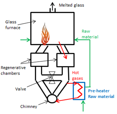
In Figure 1 a layout of the typical end-port regenerative furnace is shown with the scheme of the pre-heating system added. The raw material pre-heater is placed downstream the regeneration chamber so the residual heat of the gas can be further exploited. The pre-heater is usually a counter-current tube bundle heat exchanger where the hot gas flow from the bottom upwards and the raw material is fed at the top. The exhaust gases are released into atmosphere by a chimney.
Figure 1. Plant layout with pre-heating system
As previously described both direct and indirect pre-heater systems can be conceived. In the following sections the numerical models developed for the above systems are discussed.
3.1 Granulometry model
The first aspect to consider is the modelling of the size of the material. For simplicity, it has been assumed that the pieces of scrap glass have a parallelepiped shape of size L1×L2×S. The average length defined with the Eq. (1), neglecting the thickness S, is considered:
$L_m=\frac{L_1+L_2}{2}$ (1)
The raw material does not occupy the entire volume inside the pre-heater but a percentage is empty volume. For this reason the parameter Rg is introduced to define the ratio between the volume of glass and the total volume, Eq. (2):
$R_h=\frac{V_g}{V_T}=1-\varepsilon=1-\frac{V_g}{V_T}$ (2)
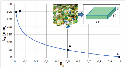
Given the size of a scrap of glass (50×50×5 [mm]), the percentage (50 %) of volume that the raw material occupy compared to the total one (Rg), it is possible to derive a relationship between Lm and Rg. This relation has been obtained by performing the regression of the curve passing for the following three points, according to the idea that in a raw material of small size the air percentage is lower than the one of the glass pieces:
A (Rg;Lm)=(0.5; 50)
B (Rg;Lm)=(0.01; 300)
C (Rg;Lm)=(0.99; 1)
The curve reported in the Eq. (3) and in the Figure 2 is obtained:
$L_m=alnR_g+b(a=-64.67;b=2.568)$ (3)
Figure 2. Relationship between the glass volume ratio and the size of the raw material
3.2 Indirect method
The preheating system with indirect heat exchange consists of a tube bundle, immersed into the raw material, where hot gas flows. The heat is transferred by conduction and radiation. In this model the raw material is treated as an equivalent solid composed of air and glass. So appropriate thermo-physical properties have been defined for the equivalent solid. For the equivalent density the mass conservation has been used, Eq. (4):
$\dot{m}_{eq}=\rho_{eq}V_T=\dot{m}_g+m_a=\rho_{g}V_g+\rho_{a}V_a=\rho_g(1-\varepsilon)V_T+\rho_{a}V_a $ (4)
in order to define the equivalent density, Eq. (5) and the equivalent conductivity, Eq. (6):
$\rho_{eq}=(1-\varepsilon)\rho_g+\varepsilon \rho_a$ (5)
$K_{eq}=(1-\varepsilon)K_g+\varepsilon K_a$ (6)
the specific heat has been calculated as the weighted average between the specific heat of glass and air, Eq. (7):
${{C}_{p,eq}}=\frac{{{m}_{g}}}{{{m}_{eq}}}{{C}_{p,g}}+\frac{{{m}_{a}}}{{{m}_{eq}}}{{C}_{p,a}}\simeq {{C}_{p,g}}$ (7)
where the specific heat of the glass (independent of the raw material size) is dominant.
3.3 Direct method
The preheating system with direct heat exchange consists of a tube bundle with several holes on the tube surface and capped on the upper surface. The exhaust gases flow through the raw material. The heat exchange takes place by not only conduction and radiation, but also by convection and higher temperatures can be reached in a shorter time. In this case a porous domain has been used, in order to model the domain containing the raw material, with the properties of the glass for the solid part and the properties of the exhaust gases for the fluid part (Cp,f=1290 [J/kgK], Kf=0.0454 [W/mK] e rf=0.53 [kg/m3]). The permeability loss coefficient C1 and the inertial loss coefficient C2 to determine the pressure drop of the exhaust gases in the porous matrix are introduced. One technique for deriving the appropriate constants involves the use of the Ergun equation [16], applicable over a wide range of Reynolds numbers and for many types of packing. This correlation has been validated in several works dealing with packed bed [17, 18], but also by the authors in applications of regenerative chambers [4, 5] and thermal storage CSP [19]. The coefficients C1 e C2 have been defined as follows, Eq. (8-9):
$C_1=\frac{1}{a}=\frac{150}{D_P^2}\frac{(1-\varepsilon)^2}{{\varepsilon }^3}$ (8)
$C_2=\frac{3.5}{D_P}\frac{(1-\varepsilon)}{ {\varepsilon }^3}$ (9)
These coefficients depend on the porosity e and on the diameter DP of the equivalent sphere of a piece of raw material that is assumed equal to Lm.
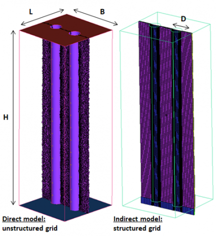
Different CFD models have been set up for both direct and indirect heating systems. Using the above models a sensitivity analysis on the properties of the raw material has been performed in order to understand the effects of the main parameters and to derive useful output for design strategies. The CFD analysis have been performed with the Ansys Fluent v.17.1 software, while geometries and grids have been generated with ICEM CFD. The simplified model consists of a representative module of a real pre-heater. Only two pipes, distant 200 [mm] from their centres, constitute the base modulus in order to save computational resources. These pipes are 1.42 [m] height and lay a rectangular base of B=500 [mm] and L=490 [mm]. The tubes have been modelled as smooth walls in the indirect case, because the exhaust gases do not get into direct contact with the raw material. In the direct case a series of small holes has been designed on the side walls of the pipes. Each tube has 52 holes of diameter d=8 [mm] on every 90° arrangement and along the height equally (4×13) distributed; the pipe top is capped. Two different meshes have been generated (Figure 3).
For the indirect case a structured multi-block grid made of O-grid blocks inside the pipes can be generated with about 0.4 Mcells. For the direct case, due to the presence of the holes, an unstructured grid with prism layer has been used with about 7 Mcells. In both cases the first wall cell size gives a Y+ close to 30. The standard k-e with scalable wall functions have been used for the turbulence closure. The transport model of chemical species has been activated for the hot gases that consist of 1 % of Argon, 9.4 % of carbon dioxide, 19 % of water vapour and the remaining part of nitrogen. The solver obtained the properties of the gases as the mixing of the individual species properties. Moreover, the radiation P1 model is considered. The buoyancy model has been used, in order to consider the free convection motions. The standard 2ND order SIMPLE numerical scheme has been activated. All the simulation performed are unsteady in order to reproduce the thermal response of the system. The time has been fixed to 5 hours to compare the effects of the different solutions. The following boundary conditions have been set: at the inlet a normal massflow rate condition of 0.0288 [kg/s], with a temperature of 730 [K] and a turbulence intensity of 5 %; at the outlet an outflow condition has been set. For the pipe wall and the base, a no slip condition has been used with a coupled heat transfer condition. The tube is designed as an infinitesimal wall that couples the gas to the raw material, while the thickness (4 [mm]) and the thermal conductivity (15 [W/mK]) are introduced into the numerical interface. A symmetry condition is introduced for the external walls of the box. The small holes in the pipe surfaces for the direct model are treated as interfaces between the fluid and the porous domain.
Figure 3. Mesh cut plane of the two simplified models
In the following sections several CFD analysis are shown to understand the effects of the main parameters and to compare the different solutions and models. The time history of the average temperature of the raw material volume is used as monitor value to compare.
5.1 Direct model
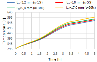
A parametric analysis has been carried out to gain a sensitivity on the impact of the main parameters on the system response. In the direct model the size of raw material (related to the porosity and consequently the porous resistance) has been varied following Eq. (8-9). Figure 4 compares the volumetric temperature trends over time for different dimensions Lm of the raw material.
It is clear that as the size of the scrap increases, the system has a faster thermal response. In fact, when the raw material is larger, there is less volume of the exchanger actually filled by raw material and the gases can find their way through the packed bed. The effect is more pronounced when e increases. A variation from e=0.1 to 0.2 gives about 5 [K] difference while a negligible temperature change is observed in the range e=0.01 - 0.1.
Figure 4. Raw material size analysis on direct model
5.2 Indirect model
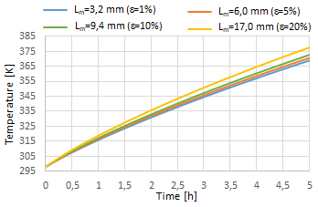
In Figure 5 the temperature trend over time are reported for different dimensions of the raw material (influence on the equivalent solid properties - density and thermal conductivity).
Figure 5. Raw material size analysis on indirect model
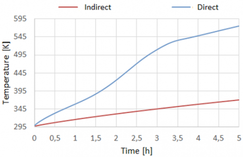
Figure 6. Comparison between the indirect and direct CFD model–thermal response
As for the direct case a quicker response is obtained by increasing the raw material size. The difference concerns the temperature values achieved in the two different thermal modes. With the same raw material properties and e=0.05 a temperature higher than 200 [K] is obtained in the direct case, at the end of the pre-heating time while, as expected, a much slower thermal response is obtained with the indirect case. The difference is quantified in the comparison of Figure 6.
The direct method is clearly more efficient than the indirect case. However, since the direct method requires appropriate filtering systems for the gases which can release harmful substances and powder, it requires special post treatment systems and it is therefore less attractive. For this reason the attention has been focused on the indirect approach in order to develop models and tools for its optimal design. Attention has been given to the individual properties of the scrap glass. In order to make the comparisons easier a baseline case has been identified (Table 1).
Table 1. Baseline case properties
|
e |
Cp,g [J/kgK] |
Kg [W/mK] |
rg [kg/m3] |
|
0.05 |
800 |
0.75 |
2575 |
Table 2 summarizes the set of cases considered with the percentage variations of the individual properties of the respective raw material.
Table 2. Dataset of cases with the properties variations
|
Case |
Parametric variation |
|
A1 |
Δrg = 4.8 % |
|
A2 |
Δrg = -10.7 % |
|
B1 |
ΔCp,g = 12.5 % |
|
B2 |
ΔCp,g = 25.0 % |
|
C1 |
ΔK,g = -20 % |
|
C2 |
ΔK,g = 20 % |
Figure 7. Raw material density analysis on indirect model
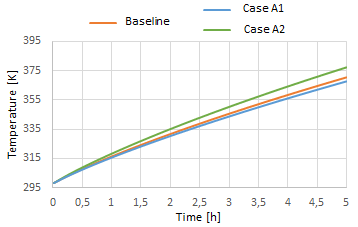
The system response by changing the raw material density is shown in Figure 7. It can be noticed that the raw material density has a modest impact on the temperature trend. The response is slower when the density increases, because the system has a greater thermal inertia; by increasing the density with respect to the baseline case of about 5 %, a lower temperature of about 3 [K] is obtained at the end of the pre-heating time. In Figure 8 the comparisons of the temperature trends with the variation of the specific heat of the raw material is reported. In this case a more marked variation is observed with respect to the density analysis. A variation of about 10 [K] is obtained with a 12,5 % change in the specific heat. If the specific heat increases, a larger amount of energy is required to get the same temperature change and a slower system response is observed.
Figure 8. Raw material specific heat effect - indirect model
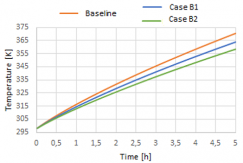
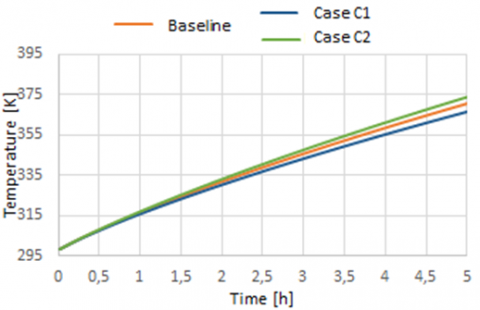
In Figure 9 the temperature trends over the time with different thermal conductivity of the scrap glass are compared.
Figure 9. Raw material thermal conductivity effect -indirect model
In this case a variation of almost 5 [K] has been highlighted by varying the conductivity of 20 %. A faster thermal response is obtained by increasing the thermal conductivity.
5.3 Energetic considerations
From the parametric analysis the impact of each individual parameter in a raw material pre-heater is identified and with the CFD model can be quantified. The designer can use the results in order to understand the impact on the energetic balance of the system (combustion fuel gain) for a given raw material characteristic. The heat flux that the fuel (methane) have to provide to the glass bath following the observed temperature change compared to the baseline case, at the end of the pre-heating time is:
$\dot{m}_Gc_{p,g}\Delta T_{baseline}=\delta q=\delta \dot{m}_{{CH}_4}Hi$ (10)
Assuming that in a generic glass furnace 356 tons/day (or 4.12 [kg/s]) of raw material to melt are introduced and that a generic glass bath absorbs 8.3 [MW] [20], the percentage variations of the fuel massflow rate can be predicted; consequently the economy savings in the furnace management can be estimated. Assuming that the percentage of recycled material is in the range 20 and 80 %, the impact on fuel is reported in Table 3, for all the cases previously simulated.
Table 3. Fuel percentage variation for the several cases
|
Case |
$\delta \dot{m}_{{CH_4}}$[%] |
|
e=0.01 |
(0.01÷0.05) |
|
e=0.1 |
- (0.02÷0.06) |
|
e=0.2 |
- (0.06÷0.22) |
|
A1 |
(0.02÷0.09) |
|
A2 |
- (0.05÷0.22) |
|
B1 |
(0.06÷0.24) |
|
B2 |
(0.12÷0.48) |
|
C1 |
(0.03÷0.13) |
|
C2 |
- (0.03÷0.10) |
From this analysis is clear that raw material of larger dimensions and high conductivity, having a low density and specific heat, is preferable. The highest influence is given by the specific heat: a fuel variation of about 0.5 % can be obtained with a specific heat change of 25 %.
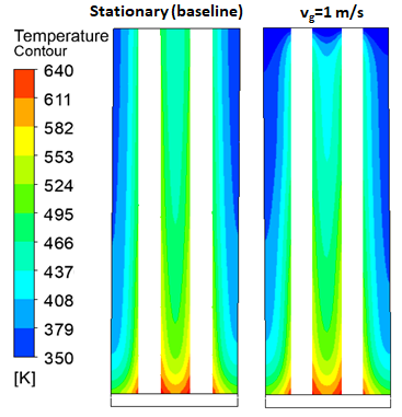
The raw material filling process in the pre-heater is carried out continuously through a hopper that on the top feeds the exchanger with the cold raw material and collects the heated material on the bottom side to feed the furnace. The relative motion between pipes and raw material has been introduced into the CFD model in order to understand the effect with respect to the previous analysis. A velocity value is imposed at the pipe walls of the exchanger with a direction parallel to their axes. In order to simulate the continuous filling of new cold raw material, a constant temperature equal to 298 [K] has been set on the upper end of the solid domain. In Figure 10 a comparison of the temperature contours for the cases of stationary domain (left) and moving domain (right) are shown and the difference in the temperature gradients can be appreciated. In Figure 11 the trends of the system responses with different raw material velocities are compared with the baseline case (stationary v=0 m/s case).
Figure 10. Comparison of the temperature contours for the stationary and the raw material motion
Only in case of high velocity, the relative motion affects the system response. With v=1.0 [m/s] a lower temperature is obtained compared to the stationary case; in fact the raw material has a shorter residence time in the pre-heater. In a glass furnace, the inlet velocity of the batch blanket is generally of the order of 0.002 [m/s] [20]. If the inlet velocity of the batch blanket is assumed comparable to the raw material velocity in the pre-heater, it evident that for this value there is practically no influence on the temperature trend over the time between the two CFD approaches.
Figure 11. Analysis with different raw material velocities
Low relative velocities between pipes and raw glass are also required for a lower mechanical erosion of the pre-heater. It can be therefore confirmed that the CFD model with no relative motion between raw glass and pipes is adequate for design purposes.
This section describes an analytical model based on the lumped parameters approach developed for a quick analysis of raw material pre-heating system in the indirect heat transfer case. The results of the analytical model are compared to those from CFD in order to tune the 0D approach. To calculate the heating rate of the raw material, the energy balance is imposed, Eq. (11). The internal energy variation of the raw glass is equal to the variation of the thermal heat flow through the system. The incoming heat flow includes the heat entering from the pipes, Eq. (12), and the heat entering from the lower and upper base of the box; the heat dispersed in the environment is clearly a loss, Eq. (13).
${{\rho }_{g}}{{V}_{g}}{{C}_{p,g}}\frac{\delta {{T}_{g}}}{\delta t}=({{q}_{tubes}}+{{q}_{bottom}}+{{q}_{top}})-{{q}_{loss}}$ (11)
${{q}_{tubes}}={{U}_{tot}}{{A}_{tubes}}({{T}_{f}}-{{T}_{g}})$ (12)
${{q}_{loss}}={{U}_{box}}{{A}_{box}}({{T}_{g}}-{{T}_{amb}})$ (13)
The upper and lower base have been neglected. The average dispersion efficiency has been introduced, Eq. (14). In this way Eq. (11) can be simplified in Eq. (15).
${{\eta }_{loss}}=1-\frac{{{q}_{loss}}}{{{q}_{tubes}}}$ (14)
${{\rho }_{g}}{{V}_{g}}{{C}_{p,g}}\frac{\delta {{T}_{g}}}{\delta t}={{\eta }_{loss}}{{U}_{tot}}{{A}_{tubes}}({{T}_{f}}-{{T}_{g}})$ (15)
The analytical solution of the previous equation is reported in the Eq. (16). It gives the temperature trend of the equivalent solid over time, where the exponent is the ratio between the time and the characteristic time of the system, as reported in Eq. (17).
${{T}_{g}}={{T}_{f}}+({{T}_{g,0}}-{{T}_{f}}){{e}^{-\left( {}^{t}/{}_{{{\tau }_{id}}} \right)}}$ (16)
${{\tau }_{id}}=\frac{{{\rho }_{g}}{{V}_{g}}{{C}_{p,g}}}{{{\eta }_{loss}}{{U}_{tot}}{{A}_{tubes}}}$ (17)
The characteristic time depends on the thermal inertia of the equivalent solid, on the tube exchange surface, on the box dispersion efficiency and finally on the transmittance (Eq. 18), that considers the conductive resistance of the tube and the internal convective resistance.
${{U}_{tot}}=\frac{1}{{}^{{{A}_{e}}}/{}_{{{A}_{i}}{{h}_{f}}}+\frac{{{A}_{e}}}{2\pi {{K}_{tubes}}L}\ln {}^{{{r}_{e}}}/{}_{{{r}_{i}}}}$ (18)
Forced convection in pipes is described by the following dimensionless parameters: Reynolds number, Eq. (19), Prandtl number, Eq. (20) and Nusselt, Eq. (21).
${{R}_{{{e}_{D}}}}=\frac{{{\rho }_{f}}{{v}_{f}}D}{{{\mu }_{f}}}$ (19)
${{P}_{r}}=\frac{{{\mu }_{f}}{{C}_{p,f}}}{{{K}_{f}}}$ (20)
${{N}_{{{u}_{x}}}}=\frac{{{h}_{f}}D}{{{K}_{f}}}=f({{R}_{{{e}_{D}}}},{{P}_{r}})$ (21)
As the flow regime inside the tubes is similar to a not fully developed motion, the correlations for the calculation of the local Nusselt number have been reported in Eq. (22), the first line is valid when
, while the second when >0.01. This regime is valid if the dimensionless abscissa, Eq. (23), respects the condition reported in Eq. (24) at the exit of the tube.${{N}_{{{u}_{x}}}}=\left\{ \begin{matrix} 1077x_{*}^{-{}^{1}/{}_{3}}-0.7 \\ 3.657+6.874{{({{x}_{\phi }}\times {{10}^{3}})}^{-0.488}}{{e}^{-57.2{{x}_{\phi }}}} \\ \end{matrix} \right.$ (22)
${{x}_{\phi }}=\frac{{}^{x}/{}_{D}}{{{R}_{{{e}_{D}}}}{{P}_{r}}}$ (23)
${{x}_{\phi }}(H)<{{\bar{x}}_{\phi }}=0.05$ (24)
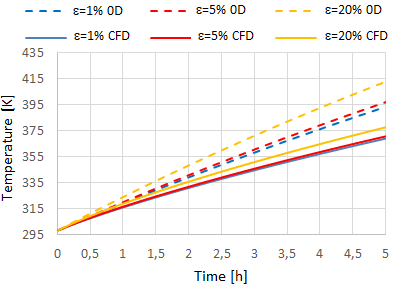
This analytical 0D model has been applied to three different sizes of raw material (different e). In Figure 12 the temperature distributions are compared to those obtained by the CFD.
Figure 12. Comparison between 0D and CFD models
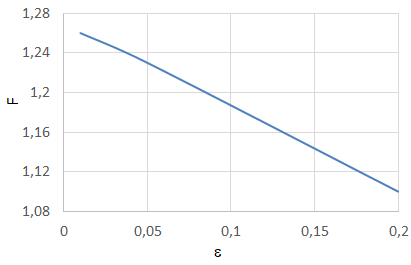
Figure 13. Correlation factor vs size of raw material
Using the above curves, a calibration factor for the 0D analytical model can be obtained. The characteristic time from CFD results has been estimated. Table 4 shows the numerical values of the calibration factors F defined as the ratio
for different size of raw material (e). Figure 13 shows the relationship between the calibration factor and the size of the raw material.The above relation is introduced to use the 0D model for quick parametric analysis for the preliminary design phases before a CFD simulation campaign.
Table 4. Calibration factors for different size of raw material
|
e |
F |
|
0.01 |
1.26 |
|
0.05 |
1.23 |
|
0.2 |
1.1 |
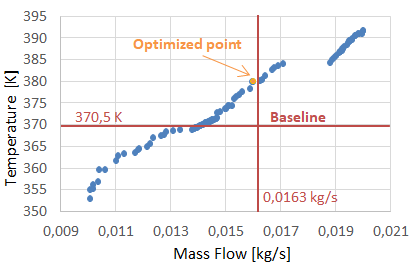
A design optimization strategy based on the response surface approach has been developed. This approach has been used for several different applications and it is very effective when the numerical simulation of the system is computationally expensive of if many design variables are considered [21]. The goal of this optimization procedure is to obtain the pipe geometry (thickness and diameter) that maximizes the final temperature of the raw material and minimizes the mass flow rate of the hot gases. A Design of Experiment (DOE) dataset of configurations has been generated with the Latin Hypercube Sampling model. The range of the parameters that define the design space is reported in Table 5. A DOE with 80 samples has been generated and validated. In Figure 14 the obtained mass flow rate from each CFD simulation (using the same CFD model and settings for indirect heat transfer previously described) of the DOE is reported (blue dots). In the same figure, the individuals generated by the optimization process (using the response surface) are also reported (red dots).
Table 5. Parameter ranges for the optimization procedure
|
D [mm] |
S [mm] |
ṁ [kg/s] |
|
80÷100 |
1÷5 |
0.01÷0.02 |
Figure 14. DOE and MOGA individuals for mass flow rate
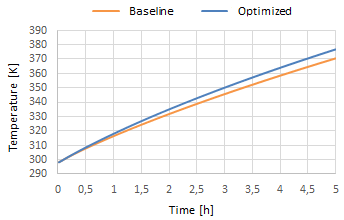
The Dakota software platform has been used for the optimization procedure. The multi-objective genetic algorithm MOGA has been used for the optimization process working on the response surfaces of the mass flow rate and of the final temperature from the heating. After a sensitivity analysis over the number of populations and generations, the MOGA has been set up with a total of 12.000 iterations to play on the response surfaces The Pareto Front obtained is shown in Figure 15. The optimum point on the Pareto Set of Figure 15 that has a lower mass flow and a higher final temperature than the reference case has been selected. The corresponding geometrical data of the optimized case are reported in Table 6. In order to validate the process a CFD simulation has been performed on the optimized configurations. The temperature trends of the optimized and baseline geometries are compared in Figure 16.
Table 6. Geometrical data of the optimized case
|
D [mm] |
S [mm] |
ṁ [kg/s] |
|
91.63 |
3.8 |
0.0162 |
Figure 15. Pareto front
Figure 16. Optimized vs baseline case
The results confirm the improvement in the optimised configuration with respect to baseline. A reduced massflow rate of 0.6% and a lighter pipe (larger diameter, and lower thickness), give a higher raw material temperature of about 7 [K]. It results in a saving of fuel for the glass furnace, but also in lower costs for the constructions of the pre-heater due to the reduction of steel needed.
Several models have been presented for the pre-heating of raw material for both direct and indirect heating processes. The attention has been actually focused on the indirect process because it is safer with respect to environmental problems related to the exhaust gases. The numerical models can be used to quantitatively compare the effects of the main design parameters taking into account the raw material dimensions and physical properties. The parametric analysis can be used either for design purposes or to support the decision making process according to the economic savings associated to the pre-heater with a given raw material and hot gas conditions.
With a reference raw material in mind, it has been estimated that a variation of 25 % of specific heat leads to a variation of 0.5 % of fuel. With the estimated fuel consumption from an average furnace [20] giving an annual cost of the order 14 M€, a saving of 70 k€ can be expected with the above solution. A lower advantage is obtained with the variation of the density and the lowest impact is predicted the change of thermal conductivity of the raw material. As far as the raw material size is concerned, it has been observed that only for values of Lm>10 [mm] there is a pronounced impact. It has been also verified that a CFD model with stationary raw material is representative and accurate because the velocity of the raw material (with values compatible with an actual design vg=0.002 [m/s]) gives no thermal effects on the system response.
An optimization procedure, based on CFD models and response surfaces, has been developed to support the design process of the system.
The present work has been supported by a funding from Regione Liguria POR FESR Liguria 2014-2020 – Asse 1 – Azione 1.2.4 CUP G38I17000010007 to support industrial research and innovation.
|
A |
area, [m2] |
|
B |
base length, [m] |
|
C1 |
permeability loss coefficient, [1/m2] |
|
C2 |
inertial loss coefficient, [1/m] |
|
Cp |
specific heat, [J/kgK] |
|
d |
hole diameter, [mm] |
|
D |
diameter, [mm] |
|
Dp |
mean particle diameter, [m] |
|
F |
calibration factor |
|
h |
convective heat transfer coefficient, [W/m2K] |
|
H |
height, [m] |
|
Hi |
lower heating value, [J/kg] |
|
K |
thermal conductivity, [W/mK] |
|
L |
width, [m] |
|
Lm |
average length of the raw material, [mm] |
|
m |
mass, [kg] |
|
ṁ |
massflow rate, [kg/s] |
|
Nu |
Nusselt number |
|
Pr |
Prandtl number |
|
q |
heat, [W] |
|
r |
radius [mm] |
|
Re |
Reynolds number |
|
Rg |
glass ratio |
|
S |
thickness, [mm] |
|
t |
time, [s] |
|
T |
temperature, [K] |
|
U |
transmittance, [W/m2K] |
|
v |
velocity, [m/s] |
|
V |
volume, [m3] |
|
x |
local coordinate, [m] |
|
Y+ |
non dimensional boundary layer distance from wall |
|
Greek symbols |
|
|
e |
porosity |
|
η |
efficiency |
|
µ |
dynamic viscosity, [Pa s] |
|
r |
density, [kg/m3] |
|
τid |
characteristic time, [s] |
|
Subscript |
|
|
0 |
initial condition |
|
a |
air |
|
amb |
ambient |
|
e |
external |
|
eq |
equivalent |
|
f |
exhaust gas |
|
g |
glass |
|
i |
internal |
|
T |
total |
[1] Zarrinehkafsh MT, Sadrameli SM. (2004). Simulation of fixed bed regenerative heat exchangers for flue gas heat recovery. Applied Thermal Engineering 24(2-3): 373-382. https://doi.org/10.1016/j.applthermaleng.2003.08.005
[2] Reboussin Y, Fourmigué JF, Marthy JF, Citti O. (2005). A numerical approach for the study of glass furnace regenerators. Applied Thermal Engineering 25(14-15): 2299-2320. https://doi.org/10.1016/j.applthermaleng.2004.12.012
[3] Koshelnik AV. (2008). Modelling operation of system of recuperative heat exchangers for aero angine with combined use of porosity model and thermos-mechanical model. Glass and Ceramics 65(9-10): 301-304. https://doi.org/10.1080/19942060.2012.11015446
[4] Basso D, Cravero C, Reverberi AP, Fabiano B. (2015). CFD analysis of regenerative chambers for energy efficiency improvement in glass production plants. Energies 8: 8945-8961. https://doi.org/10.3390/en8088945
[5] Cravero C, Marsano D. (2017). Numerical simulation of regenerative chambers for glass production plants with a non-equilibrium heat transfer model. WSEAS Transactions on Heat and Mass Transfer 12(3): 21-29.
[6] Cravero C, Marsano D, Spoladore A. (2017). Numerical strategies for fluid-dynamic and heat transfer simulation for regenerative chambers in glass production plants. NAUN International Journal of Mathematical Models and Methods in Applied Sciences 11: 82-87.
[7] Cogliandro S, Cravero C, Marini M, Spoladore A. (2017). Simulation strategies for regenerative chambers in glass production plants with strategic exhaust gas recirculation system. 11th AIGE 2017, 2nd AIGE/IEETA Int. Conf., 12-13 June 2017, Genova, Italy – International Journal of Heat and Technology, ISSN: 0392-8764, 35(1): S449-S445, https://doi.org/10.18280/ijht.35Sp0161
[8] Sweo BJ, Ginther JH. (1965). Method for raw material pre-heating for glass melting U.S. Patent 3 185 554.
[9] Nesbitt JD, Fejer ME. (1974). Process for pre-treating and melting glassmaking materials. U.S. Patent 3 788 832.
[10] Suzuki T, Murao M, Utiyama S, Hatanaka K, Inoue H. (1979). Premelting method for raw materials for glass and apparatus relevant thereto. U.S. Patent 4 135 904.
[11] Selvaray J, Varun VS, Vignesh, Vishwam V. (2014). Waste heat recovery from metal casting and scrap preheating using recovered heat. Procedia Engineering 97: 267-276. https://doi.org/10.1016/j.proeng.2014.12.250
[12] Nakano H, Uchida S, Arita K. (1999). New Scrap Preheating System for Elecrtic Arc Furnace (UL-BA). Nippon Steel Technical Report (79).
[13] Mandal K. (2010). Modeling of scrap heating by burners. PhD Thesis, Department of Materials Science and Engineering, McMaster University, Hamilton, Ontario, Canada.
[14] Pariona MM, Mossi AC. (2005). Numerical Simulation of Heat Transfer During the Solidification of Pure Iron in Sand and Mullite Molds. J. of the Braz. Soc. Of Mech. Sci. & Eng. XXVII (4): 399-406. https://doi.org/10.1590/S1678-58782005000400008
[15] Cravero C, Leutcha P, Mola A, Nilberto A, Spoladore A. (1952). Experimental and numerical investigations on pre-heating systems for recycled glass in glass production plants. in preparation Ergun, S., Fluid Flow through Packed Columns Chem. Eng. Prog 48(2): 89-94.
[16] Xu Z, Woche H, Specht E. (2009). CFD Flow Simulation of Structured Packed Bed Reactors with Jet Injections. The 14TH International Conference on Fluid Flow Technologies, Budapest, Hungary, pp. 536-544.
[17] Mohammadpour K, Woche H, Specht E. (2017). CFD simulation of parallel flow mixing in a packed bed using porous media model and experiment validation. Journal of Chemical Technology and Metallurgy 52(3): 475-484. https://doi.org/10.1007/s40571-018-0203-x
[18] Mahmood M, Traverso A, Traverso AN, Massardo AF, Marsano D, Cravero C. (2018). Thermal energy storage for CSP hybrid gas turbine systems: Dynamic modelling and experimental validation. Applied Energy 212: 1240-1251. https://doi.org/10.1016/j.apenergy.2017.12.130
[19] Madivate C, Muller F, Wilsmann W. (1998). Calculation of the theoretical energy requirement for melting technical silicate glasses. Journal of the American Ceramic Society 81: 3300-3306. https://doi.org/10.1111/j.1151-2916.1998.tb02771.x
[20] Cravero C, Macelloni P, Briasco G. (2012). Three-dimensional design optimization of multi stage axial flow turbines using an RSM based approach. Asme paper GT2012-68040, Asme Turbo Expo, Copenhagen (DK). https://doi.org/10.1115/GT2012-68040