Olawale Oluwasegun Ogunrinola* | Isaiah Opeyemi Olaniyi | Segun A. Afolabi | Gbemiga Abraham Olaniyi | Olushola Emmanuel Ajeigbe
© 2021 IIETA. This article is published by IIETA and is licensed under the CC BY 4.0 license (http://creativecommons.org/licenses/by/4.0/).
OPEN ACCESS
Modern radio communication services transmit signals from an earth station to a high-altitude station, space station or a space radio system via a feeder link while in Global Systems for Mobile Communication (GSM) and computer networks, the radio uplink transmit from cell phones to base station linking the network core to the communication interphase via an upstream facility.
Hitherto, the Single-Carrier Frequency Division Multiple Access (SC-FDMA) has been adopted for uplink access in the Long-Term Evolution (LTE) scheme by the 3GPP. In this journal, the LTE uplink radio resource allocation is addressed as an optimization problem, where the desired solution is the mapping of the schedulable UE to schedulable Resource Blocks (RBs) that maximizes the proportional fairness metric. The particle swarm optimization (PSO) has been employed for this research. PSO is an algorithm that is very easy to implement to solve real time optimization problems and has fewer parameters to adjust when compared to other evolutionary algorithms. The proposed scheme was found to outperform the First Maximum Expansion (FME) and Recursive Maximum Expansion (RME) in terms of simulation time and fairness while maintaining the throughput.
Global System for Mobile Communications (GSM), Long-Term Evolution (LTE), Third Generation Partnership Project (3GPP), First Maximum Expansion (FME), Recursive Maximum Expansion (RME)
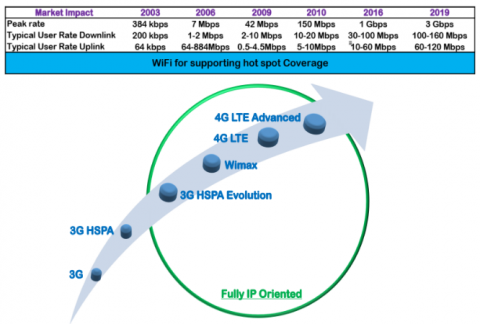
Mobile communication continues to simplify human day-to-day technological interactions and the bridge of smart business dichotomy, as well as innumerable engineering enterprise through various communication infrastructures. Over the last decades, the services provided to mobile users has been more complex and the mobile telecommunications systems must evolve to meet these expectations. The Long-Term Evolution (LTE) has been specified by the Third Generation Partnership Project (3GPP) as the new radio access technology (RAT) and network architecture for providing considerable performance improvement at a reduced cost [1]. Figure 1 is a chart showing the global mobile subscribers and market share by technology.
Figure 1. Global mobile subscribers and market share by technology
LTE has taken a giant leading leap in the domain of preferred telecommunication network interface is a next generation mobile system standard from the 3GPP which is focused on wireless broadband and represents basically an evolution of the mobile communications standards, such as UMTS and GSM. It provides throughputs up to 50 Mbps in uplink and up to 150 Mbps in downlink as standard. It uses scalable bandwidth from 1.4 to 20 MHz that suits the needs of the different network operators and its bandwidth allocations differ. Its air interface is based on: Orthogonal Frequency Division Multiple Access (OFDMA) in the downlink (with High PAPR which is undesirable for the mobile end) and Single-Carrier Frequency Division Multiple Access (SC-FDMA) in the uplink (with Low Peak-to-Average Power Ratio (PAPR), but it maintains the properties of OFDMA) [2].
LTE is now the fastest growing mobile system technology and many regions around the world are either testing or deploying this network as consumers prefer the option of a faster mobile broadband. 2017 mobile subscriber statistics showed that the number of LTE subscribers around the globe was close to 1.2 billion. LTE subscriptions are expected by forecast to have climbed to over 4.5 billion by 2020. This forecast is well on track with 422 commercial networks already in operation and 3.16 billion subscriptions as of March, 2018 [3]. There is no doubt that LTE would set a new pace and is set to take a leading role in broadband developments. With innovative smart phones, competitively priced services coupled with an increasing range of very innovative apps, the market is set to continue to boom. The technology evolution of LTE is shown in Figure 2.
Figure 2. 3GPP technology evolution
To reach LTE's design goals set by the 3GPP, LTE's new RAT and network architecture must be exploited when addressing the Radio Resource Management (RRM) design problem. RRM functionalities include Admission Control (AC), Packet Scheduling (PS) (including Hybrid Automatic Repeat Request (HARQ)), Fractional Power Control (FPC) and fast Link Adaptation (LA) (which includes Adaptive Modulation and Coding (AMC)). The RRM design problem can be summarized as providing these functionalities under the constraints introduced by the used technology such as contiguity constraint of SC-FDMA, and the constraints introduced by the design goals such as improving spectral efficiency and QoS provisioning [4, 5].
At the access level, LTE network consists mainly of LTE base stations (BSs), termed as evolved NodeBs (eNodeBs). Mobile Switching Centre and Radio Network Controller (RNC) units that are present in 2G and 3G access networks respectively have been eliminated in LTE standard. MSC and RNC units perform higher-level management of radio access network, such as mobility management and RRM. eNodeB has inherited some of RNC's responsibilities, such as RRM and mobility management, while the other tasks have been moved up to the packet core network. RRM plays a very important role in LTE networks by managing the limited radio resources such that the achievable data rates over LTE’s radio interface become as high as possible [6, 7]. The focus of the work presented here is on a very crucial RRM component residing at the eNodeB, which is the packet scheduler. The packet scheduler in LTE is responsible for allocating shared radio resources among User Equipments (UEs).
Designing a scheduling algorithm for the LTE uplink is very complex given the many constraints and numerous scheduling patterns to examine which make most existing traditional schemes unsuitable for handling these problems. Since 3GPP has not standardized any scheduling algorithm, an algorithm that would meet the expected fairness and QoS needs to be designed and implemented [8]. This research has chosen a new approach for the LTE uplink scheduling and has adopted a search algorithm that traverses the space of possible solutions in order to identify the optimum or a sub-optimum. In order to make decisions along the search path, the algorithm required an optimization measure, which is known as a metric. The metric is designed considering different scheduling aspects including channel gain, QoS requirement and fairness [9].
In 2004, 3GPP launched the Release 8 of mobile broadband standard as a burgeon of 3G solution and named it Long term Evolution. LTE comes with an enhanced features and technological edge above its 3G predecessors, and it establishes a more competitive mobile evolutionary broadband networks such as cable and Asymmetric Digital Subscriber Line (ADSL) [8]. In 2008, an additional attribute demonstrating structural access level and core level was incorporated into Release 8, and furthermore, in 2009 added advanced enhancement features to LTE to form 3GPP Release 9. LTE is of recent experiencing commercial patronization with global research investigation to maximize its capacity and improve LTE performance [8, 9].
The downlink (DL) OFDMA framework is woven to achieve high spectrum scalable bandwidth (BW) supplying high peak data rates is the technology adopted by LTE. For peak data rates close to 10 Mbps in 5 MHz of BW, WCDMA radio technology provides a twin efficiency as OFDMA.
FDMA guarantees a visible implementation advantage among infeasibility in current technology in the midst of appreciable complex terminals required in achieving peak rates of about 100 Mbps with wider radio channels [10]. OFDM is flexible in channelization and its LTE executes operation in various radio channel sizes, which ranges from 1.4 to 20 MHz. LTE has downlink peak data rates of about 150 Mbps with a bandwidth of 20 MHz and for the uplink, the peak data rates of about 50 Mbps with a bandwidth of 20 MHz Closely spaced carriers with reduced data rate modulation engages the template of OFDMA’s format. The orthogonality of this signals, cancels the propensity for mutual interference [10, 11].
2.1 Single Carrier-Frequency Division Multiple Access (SC-FDMA)
OFDMA has been selected for DL transmission in LTE because it improves spectral efficiency, provides better protection against frequency selective fading and reduces the inter symbol interference. Its high PAPR is however a disadvantage in the UL. The battery life is one of the crucial parameters that affect all mobiles. Even though there is continuous improvement in battery performance from time to time, it is still necessary to make sure that UEs consumes as little power as possible. With the radio frequency (RF) power amplifier that sends the RF signal through the antenna to the base station (BS), being the highest power device within the UE, it is important that it operates efficiently as much as possible. This can be significantly influenced by the format of RF modulation and signal. Signals with a high PAPR and require linear amplification do not lend themselves to the use of efficient RF power amplifiers. As a result, it is crucial to adopt a mode of transmission whose power level is near constant when operating [12, 13].
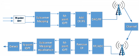
Unfortunately, OFDM has a high PAPR. While this is not a challenge for the base station where power is a small issue, it is unacceptable for the mobile device. As a result, LTE makes use of a modulation scheme, which is known as SC-FDMA, which is a hybrid format but has a 2 to 6 dB PAPR advantage over the OFDMA format used by other technologies such as WiMAX (Worldwide Interoperability for Microwave Access). It combines the multipath interference resilience and flexible subcarrier frequency allocation that OFDM offers to the low PAPR, which the single-carrier systems provided. Figure 4 is the block diagram of the SC-FDMA.
SC-FDMA also known as DFT spread OFDMA has therefore been selected for the uplink transmission (Figure 3 shows the comparison between SC-FDMA and OFDMA). In this case the subcarriers, due to the DFT-spread operation, are transmitted sequentially rather than in parallel thus resulting in a lower PAPR than OFDMA signals. This produces a higher Inter Symbol Interference (ISI) which the eNodeB has to cope with via frequency domain equalization. Thus, the SC-FDMA, while still retaining most of the benefits of OFDMA, offers improved coverage and reduced power consumption. On the other hand, it requires the sub-carriers allocated to a single terminal to be contiguous.
Figure 3. SC-FDMA block diagram [14]
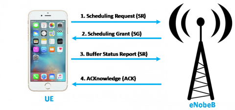
Figure 4. Scheduling process
2.1.1 Scheduling Request (SR)
UE sends a SR to notify BS that it has data to transmit and Scheduler assigns initial resources. The scheduler needs to know about the amount of data waiting transmission from terminals in order to assign proper amount of frequency resources accordingly. Obviously, there is no need to provide uplink scheduling resources to a terminal which has no data to transmit. Thus, as a minimum, the scheduler needs to obtain the knowledge of whether or not a terminal has data to send in their buffer. This is known as scheduling request.
2.1.2 Scheduling Grant (SG)
A scheduling grant contains information about the transport format to be used in addition to the information about the RBs. After the scheduling request is sent by the UE, the eNodeB replies with a scheduling grant to the UE. If the terminal does not receive a scheduling grant till the next scheduling request sub-frame, it will re-send it again. The UE is only allowed to transmit on the UL-SCH if it receives a valid grant.
2.1.3 Buffer Status Report (BSR)
This informs the eNodeB that the amount of data the user has to send is within a predefined range. When UE receives the scheduling grant, it sends BSR to eNodeB. A scheduling decision is made based on the buffer estimation. In the uplink grant, resources allocation plan, transport-block size, modulation scheme, and transmitting power are included. Among these, in order for scheduler to make the right decision on selecting transport format, the accurate information about terminal situation such as buffer status and power availability is required. After receiving a grant, the UE is allowed to transmit on assigned uplink resources. The scheduler needs information about the buffer situation in order to make appropriate decisions about the amount of scheduling resources to grant in future sub-frames. This information is supplied to scheduler during uplink transmission by the UE through the MAC control element [15-17]. The first uplink transmission will include a buffer report in most cases.
2.1.4 ACKnowledgment (ACK)
ACK indicates to the UE whether the eNodeB correctly received uplink user data carried on the PUSCH as shown in Figure 7. Several researches on LTE scheduling have been focused on the downlink. Examples of these are the ones proposed in the studies [18-23]. Many other researchers have made proposals on the LTE uplink scheduling, considering some of the challenges that concerns it. Few of these are the UE power limitation and contiguity of resource allocation. The methods of performance assessment that different researchers employ to assess their proposed schemes are most times not the same, which makes it unfair to just claim that an uplink packet scheduler outperforms another [9].
2.2 Particle Swarm Optimization (PSO)
PSO is a novel evolutionary computation algorithm, developed by Eberhart and Kennedy in 1995. Further studies in recent years have made PSO attracts much attention. This is due to its many advantages including its ease of implementation and simplicity [24]. It is a population-based, self-adaptive and swarm intelligence technique that models social behavior to guide swarms of particles towards the most promising regions of the search space. It has been proved to be efficient at solving engineering problems [25].
The advantages of the PSO algorithm include [24]:
2.2.1 PSO Description
The basic idea of PSO is as follows:
The algorithm is first initialized with the particles placed at random positions. The search space is then explored to find better solutions. In every iteration, each of the particles adjusts its velocity to follow two best solutions. The first of the solutions is the cognitive part, where each of the particles follows its own best solution that has been found so far. This is the solution that yields the highest fitness. This value is known as pBest (particle best). The second-best value is the best solution by any of the particles in the swarm, i.e., current best solution of the swarm. This value is known as gBest (global best) [26]. Each particle then adjusts its position and velocity with the following equations [27]:
The location of the ath particle:
$X_{a}=\left(x_{a 1}, \ldots, x_{a d}, \ldots, x_{a D}\right)$ (1)
The previous best position, i.e., the ath particle best fitness
$P_{a}=\left(p_{a 1}, \ldots, p_{a d}, \ldots, p_{a D}\right)$ (2)
The index of the best pBest among all the particles is represented by the symbol g. The location pg is also called gBest [28].
The ath particle velocity:
$V_{a}=\left(v_{a 1}, \ldots, v_{a d}, \ldots, v_{a D}\right)$ (3)
$v_{a d} \leftarrow w \times v_{a d}+c_{1} \times \operatorname{rand}(\cdot) \times\left(p_{a d}-x_{a d}\right)$$+c_{2} \times \operatorname{rand}(\cdot) \times\left(p_{g d}-x_{a d}\right)$ (4)
And,
$x_{a d} \leftarrow x_{a d}+v_{a d}$ (5)
where, c1 and c2 are acceleration constants, w is the inertia weight, $\operatorname{rand}(\cdot)$ is a random function in the range [0, 1].
Velocity clamping is further used to prevent the particle from moving too far away from the search space, the limits is confined to: [–Vmax, Vmax] given that the search space spans from: [–Pmax, Pmax] [28-35].
2.2.2 First Maximum Expansion (FME)
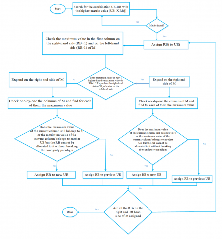
Figure 5 shows the flowchart of the FME resource allocation.
Figure 5. Flow chart of first maximum expansion [36]
The following are the steps taking in FME to allocate resources [36]:
One: Search for the combination UE-RB with the highest metric value (UE0-RB0).
Two: Assign UE0 to RB0.
Three: Check the maximum value in the first column on the right-hand side (RB+1) and on the left-hand side (RB-1) of M.
Four: If the maximum value in (RB+1) is higher than the maximum value in (RB-1), expand on the right-hand side of M, otherwise on the left-hand side.
Five: Check one-by-one the columns of M and find for each of them the maximum value. Assign the RB to the previous UE if (a) The maximum value of the current column still belongs to it; or (b) The maximum value of the current column belongs to another UE but the RB cannot be allocated to it without breaking the contiguity paradigm. Otherwise, assign it to the new UE.
Six: Repeat Step five until all the RBs on the right-hand or left-hand side of the maximum found in Step one are assigned.
Seven: In case not all the RBs have been allocated, repeat Step five and Step six in the opposite direction.
Where the subscript “0“represents the start position, i.e. M, “+” is the right-hand-side of M and “-” is the left hand side of M.
2.2.3 Recursive Maximum Expansion (RME)
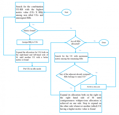
Figure 6 shows the flow chart of the RME resource allocation.
Figure 6. Flow chart of recursive maximum expansion [36]
The following are the steps taking in RME resource allocation algorithm [32]:
One: Search for the UE and RB that has the highest metric and allocate the RB to the UE.
Two: Expand the resource allocation in the first step for UE both on the right-hand and left- hand side of RB until another UE with a better metric is found.
Three: Delete the corresponding columns (RBs) and row (UE).
Four: Repeat Step one to Step three for the resulting sub-matrix. If all rows (UEs) have been deleted from matrix and not all RBs have been allocated, allocate the remaining RBs among UEs with the highest metric value but retaining the contiguity.
Five: Repeat Step four until all RBs have been allocated.
2.3 Penalty function
The most common approach in handling constraints (especially, inequality constraints) in the evolutionary algorithm (EA) community is to make use of penalties. Penalty function was proposed originally by Richard Courant in 1940 and Fiacco & McCormick and Carroll later expanded it. The penalty functions transform the constrained optimization problem into an unconstrained one simply by subtracting a certain value from the objective function or adding to it, considering in a certain solution, the amount of constraint violation present [37].
The technique based on penalty functions is the most common approaches, because of their easy application and simplicity. They depend on penalizing individuals that are out of the feasible domain. This is to make the feasible point better than the infeasible point of comparable fitness. Two main questions however arise and pose a challenge in penalty-based method [38]:
To avoid the two problems mentioned above, the penalty weights must be tuned very carefully. A small penalty level yields a solution which is not feasible (few penalized points may still possess penalized fitness that are better than the best feasible point). However, penalty levels that are high restrict the search inside the feasible region, preventing any short-cut across the infeasible region and therefore unable to converge to the optimal solution eventually [38].
2.4 LTE simulator
There are several LTE simulators, some of which include: NS Simulator, LTE Simulator, glomosim, Link Level Simulator and LTE-Sim. At the present, most of the open source simulation platforms that are useful to the scientific community to evaluate the performance of the whole LTE system are not readily available. The scarcity of a common reference simulator does not aid the work of researchers and poses limitations on the comparison of results published by different groups of research. To resolve this issue, LTE-Sim which is a open source framework is delivered to supply a complete performance verification of LTE systems. Written as an event-driven simulator in C++ language using object-oriented paradigm. LTE-Sim was conceived to simulate UL and DL scheduling strategies in multi-cell/multi-user environments, taking into account radio resource optimization, user mobility, AMC module, frequency reuse techniques and other aspects that are relevant to the scientific and industrial communities. Its main classes handle network devices, protocol stack entities, layer and network topology. The effectiveness of this simulator has been tested and verified looking at [39]:
In creating a basic scenario, the following criteria should be followed [38]:
Create four basic LTE-Sim components (network manager, frame manager, flow manager and the simulator).
3.1 Scheduling model
In LTE an RB consists of 12 subcarriers. This research uses the PF criterion with a scheduling metric value obtained from the value of each UE’s RB. The PF criterion is very important for a fair allocation available UEs. Throughput and fairness are considered when allocating resources to available UEs. Figure 7 shows a two-dimensional array table that consists of PF metrics M generated by each of the UEs and RBs at every time slot interval.
Figure 7. User Equipment (UE) to Resource Block (RB) mapping
Assuming that the scheduler is capable of assigning RBs arbitrarily to all users and each RBj has a bandwidth of $(B /|\mathbb{J}|).$ Where $\mathbb{J}$ denote Set of RBs.
The maximization problem is developed considering the proportional fair algorithm and the LTE uplink scheduling model. The objective is to maximize the limited available resource blocks while satisfying the channel orthogonality constraint, allocation contiguity constraint, power constraint and scheduling time constraint.
The proportional fair maximization at each time slot can be written as:
$M_{i, j}=r_{i, j}(t) / R_{i}(t)$ (6)
where:
$r_{i, j}=$ Instanteneous data rate for user ion RB $j$, and $R_{i}=$ Long $-$ term data rate of user $i$.
Formal definition of scheduling model:
Maximize $\sum_{i \in \mathbb{N}} \sum_{j \in \mathbb{J}} M_{i, j} A_{i, j}$ (7)
$A_{i, j}=\left\{\begin{array}{l}1 \text { if U Eiisallocatedto RBj } \\ \text { 0 otherwise }\end{array}\right.$ (8)
S.T
$\sum_{i \in \mathbb{N}} A_{i, j} \leq 1, \forall j \in \mathbb{J}$ (9)
$A_{i, j}-A_{i,(j+1)}+A_{i, k} \leq 1$, for $k=j+2, j+3, \ldots|\mathbb{J}|$ (10)
$\sum_{i \in \mathbb{J}} P_{i, j} A_{i, j} \leq m_{i}, \forall i \in \mathbb{N}$ (11)
$\sum_{j \in \mathbb{J}} t_{i} A_{i, j} \leq u, \forall i \in \mathbb{N}$ (12)
Eq. (6) through (12) are described as follows:
Eq. (6) is the throughput performance index of user i when assigned RBj;
Eq. (9) shows the orthogonality of the users within the same cell (It means a particular RB can be assigned to only one UE;
Eq. (10) shows the allocation contiguity for user i as provided by SC-FDMA in the LTE uplink;
Eq. (11) shows Power constraint; and
Eq. (12) shows Time constraint.
where:
Mi,j= Metric for user i and RBj,
$\mathbb{N}$= Set of User Equipments,
$\mathbb{J}$= Set of Resource Blocks,
u= Allowable deadline for a user,
mi = Maximum power allocation for user i.
Ai,j= Assignment variable,
ti= Allocation time for each user i,
Pi,j= Power allocated to RBj used by user i.
3.2 Penalty factor
The particles with violated constraints need to be penalized. The motive behind this is to reset the velocity of the violating particles [40]. The fitness function for each of the users can be evaluated as:
$\begin{aligned} \text { Maximize } H(\mathrm{~A})=& M+w_{1} \omega+w_{2} \Phi+w_{3} \beta \\ &+w_{4} \alpha \end{aligned}$ (13)
where, $w_{1}, w_{2}, w_{3}$, and $w_{4}$ refers to the penalty terms weights.
Penalty for violating orthogonality constraint:
$\omega=\sum_{i \in \mathbb{J}} \max \left(0, \quad 1-\sum_{i \in \mathbb{N}} A_{i, j}\right)$ (14)
Penalty for violating contiguity constraint:
$\Phi=\max \left(0, \quad 1-\sum_{i \in \mathbb{N} j \in \mathbb{J}}\left(A_{i, j}-A_{i,(j+1)}+A_{i, k}\right)\right)$ (15)
Penalty for violating power constraint:
$\beta=\sum_{i \in \mathbb{N}}\left(m_{i}-\sum_{j \in \mathbb{J}} P_{i} A_{i, j}\right)$ (16)
Penalty for violating time constraint:
$\alpha=\sum_{i \in \mathbb{N}}\left(\max \left(0, u-\sum_{j \in \mathbb{J}} t_{i} A_{i, j}\right)\right)$ (17)
3.4 PSO based radio resource scheduling algorithm
All resource block schemes were mapped onto a group of search space particles. Each particle represents a scheme, and the particle position given as [41]:
$X_{a}=\left(x_{a 1}, \ldots, x_{a j}, \ldots, x_{a|\mathbb{J}|}\right)$ (18)
Eq. (18) is the dimension of the schemes. Only one scheduling block may be allocated to one user. If the system has $|\mathbb{J}|$ scheduling blocks and $|\mathbb{N}|$ users, scheduling block’s chosen user must be [1,i]. So the particle coordinate has $|\mathbb{J}|$ dimensions, and each dimension’s value is an integer from 1 to $|\mathbb{N}|$. The velocity of the particles in the swarm is given by [41]:
$V_{a}=\left(v_{a 1}, \ldots, v_{a i}, \ldots, v_{a|\mathbb{J}|}\right)$ (19)
which stands for the particle developing direction.
The next step is the derivation of the fitness function H(A) which has been shown previously in Eq. (1-5).
The final step is the update of the particle’s position. Each of the particles in the swarm will update its velocity and position:
$P_{a}=\left(p_{a 1}, \ldots, p_{a j}, \ldots, p_{a|\mathbb{J}|}\right)$ (20)
and global best position
$P_{g}=\left(p_{g 1}, \ldots, p_{g i}, \ldots, p_{g|\mathbb{J}|}\right)$ (21)
The velocity update function is given as:
$v_{a j} \leftarrow w \times v_{a j}+c_{1} \times \operatorname{rand}(\cdot) \times\left(p_{a j}-x_{a j}\right)$$+c_{2} \times \operatorname{rand}(\cdot) \times\left(p_{g j}-x_{a j}\right)$ (22)
and
$x_{a j} \leftarrow x_{a j}+v_{a j}$ (23)
rand $(\cdot)$ is a random function that falls between the range [0, 1], where w is the inertia weight, c1 and c2 are acceleration constants or learning factors. These make every particle have ability to learn from group’s excellent particle position pgj and its history excellent position paj in order to move closer to a more outstanding position [41].
In the search process, the particles remember their experience while making reference to the experience of their peers [42].
The particle swarm resource allocation algorithm may therefore be summarized as:
Each dimension d of the particle a is updated by using Eq. (23).
$x_{a d}=\left\{\begin{array}{l}1 \text { rand }(\cdot)<S\left(v_{a j}\right) \\ 0 \text { otherwise }\end{array}\right.$ (24)
The velocities are mapped to the probabilities by the use of sigmoid function defined as [43]:
$S\left(v_{a j}\right)=\frac{1}{1+e^{\left(-v_{a j}\right)}}$ (25)
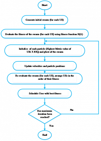
Figure 8. Flow diagram of the scheduling algorithm
Because simulations are not precise, a single simulation run is usually inaccurate and produces ambiguous conclusions. However, multiple simulation runs provide credibility and relative accuracy. Therefore, for the sake of statistical validity of the simulations, the Monte- Carlo simulation was used. At each Monte-Carlo run, the power of each UE and data transmission randomly generated to simulate the fact that users may be in separate locations. The results of simulation are averaged over 10 Monte-Carlo run.
In this analysis, the proposed scheme, PSO based radio resource scheduling algorithm (PSO), was compared with two well-known traditional scheduling algorithms such as the First Maximum Expansion based radio resource scheduling algorithm (FME) and the Recursive Maximum Expansion based radio resource scheduling algorithm (RME). The comparison was carried out in terms of system throughput, fairness and simulation time.
4.1 Simulation parameters
LTE uplink simulation was performed by implementing the PSO based radio resource scheduling algorithm on the LTE-Sim to evaluate the performance of the propose scheduling scheme. Simulation was carried out using a Linux machine with a 2.2 GHz CPU and 2 GBytes of RAM. Figure 8 shows the flow diagram of the scheduling algorithm and its adoption for simulation analysis.
Table 1 summarizes the parameter settings in the simulator for the LTE uplink scheduling algorithm.
Table 1. Parameter settings
|
PARAMETERS |
SETTINGS |
|
System Bandwidth (MHz) |
20 |
|
Subscriber per RB |
12 |
|
RB bandwidth (kHz) |
180 |
|
Number of RBS |
96 |
|
eNB: Power transmission |
43 dBm uniformly distribute |
|
Cell-level user distribute |
Uniform |
|
Number of active users in cell |
10,20,30,40,50,60 |
|
Traffic Model |
Real time traffic type: H264, VoIP |
|
UE mobility model |
Random Directions |
|
Transmission time interval (TTI)(ms) |
1 |
|
User speed (km/h) |
3,30,120 |
|
User receiver |
1x2/MMSE/ZF |
|
Modulation coding rate settings |
QPSK: 1/3, 1/2, 2/3, 3/4, 16QAM: 1/2, 2/3, 3/4 |
|
HARQ Ack/Nack delay (ms) |
8 |
|
PSO Settings |
Number of practice = 50, w = 0.7298, C1 = 1.496 and C2 = 1.496 |
The schedulers’ performances are demonstrated through computer simulation and the result of simulation are graphically shown and discussed.
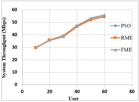
4.1.1 System throughput
It was observed from Figure 10 that system throughput performance increased in all the schemes as the number of UEs increases, as a result of multi-user diversity gain increase. Also, in PSO, Fist Maximum Expansion (FME) and Recursive Maximum Expansion (RME), their throughput levels were almost the same at the point when the number of users in the system is between 10 to 20 after which both PSO and FME showed a noticeable improvement with respect to RME. PSO and FME exhibit relatively similar performance levels until the number of users reaches 35. FME performed relatively best. Thus, the performance gap between the developed scheme and the two other traditional schemes is not a wide one.
Figure 9 illustrates the system throughput (Mbps) with respect to the number of UEs with PSO representing the proposed scheme.
Figure 9. System throughput
4.1.2 Fairness index
The Jain’s fairness index was used to measure the fairness of all the schemes.
Jain’s fairness index is introduced to measure fairness in the distribution of RBs among UEs.
$J=\frac{\left|\sum_{i \in \mathbb{N}} R_{i}\right|^{2}}{|\mathbb{N}| \cdot \sum_{i \in \mathbb{N}} R_{i}^{2}}$ (26)
where, J is the Jain’s fairness index and $R_{i}=$ Long - term service rate of user $i$ (Jain’s Index returns a number between 0 and 1, with 1 being perfectly fair [44]).
Figure 10. Jain's fairness index
Figure 10 illustrates the fairness index with respect to the number of UEs. All the schemes produce a relatively fair resource allocation scheme. A decrease in fairness was observed as the number of user increases. As the number of users in the system increases, there are more users with bad and good channel conditions. There is therefore an increase in the level of competition by UEs for the available resources in the network. This means that as number of UEs increases, the probability of omitting more users also increases. The fairness index is therefore reduced. PSO performed relatively better than RME and FME in terms of fairness. As the fairness is dependent on per UE mean throughput, therefore, the proposed algorithm is not expected to perform lesser with respect to fairness. It can also be observed that RME is marginally better than FME when the number of UEs is small, but as the number of UEs increases, they tend towards close fairness value until they intercepted at 50 users. Figure 11 also shows how they interface with the system based on fairness index and system throughput.
Figure 11. Relationship between simulation time and number of users
4.1.3 Simulation time
Figure 12 reports the simulation time with respect to the user’s number. The simulation time depends almost linearly on the number of UEs in all cases. Increasing the number of users influences the overall running time, as computing the system parameters requires more operations. The PSO algorithm requires less time than the other scheduling strategies due to its very simple implementation and fewer parameters.
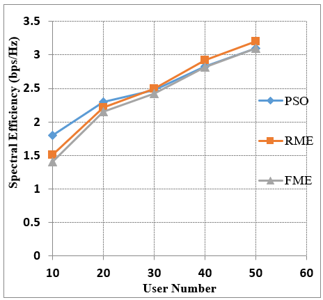
Figure 12. Relationship between average spectral efficiency and number of users
4.1.4 Spectral efficiency
Figure 12 shows the spectral efficiency with respect to number of users. It was observed that as the number of UEs increases, the spectral efficiency also increases. This is because of the multi-user diversity gain property of LTE system. RME shows a better performance than FME because of the recursive search of the RME metrics, which leads to higher scheduling gain. The gain of PSO is appreciable over RME just until 25-30 users. For higher number of users, PSO and FME perform equivalently and RME performs a bit relatively better than the other schemes [45-48].
4.1.5 Speed of convergence
During simulation, it was observed that the particle number plays a very crucial role in the experiment to prevent the PSO from early convergence and slow convergence. Figure 12 and 13 illustrate the average objective values that resulted from the simulation. Figure 13 shows the relationship between the number of iterations and number of particles to be a linear one. As number of particles increases, the result becomes better, but at a cost of more fitness evaluations, but there is a threshold beyond which the results will not be affected in a significant manner as shown in Figure 13. If number of particles is too small, the solution region covered at each iteration is not enough so the result will be poor. Considering both the search quality and computational complexity, it is recommended to choose number of particles just after the convergence. This falls between 50 and 70. 50 Particles was used in this research.
Figure 14 also shows the point of convergence which is around 1.7736.
Figure 13. Relationship between number of iterations and number of particles
Figure 14. Relationship between fitness function and number of particles
In this research, a PSO-based radio resource scheduling algorithm has been developed for the LTE Uplink. By comparing all results gathered from the three different algorithms, it can be observed that PSO performed the best out of the three schemes, this can be explained by studying how these algorithms work. RME algorithm recursively finds the maximums then iteratively allocates resources on its right- and left-hand sides, and then recurs, but PSO intelligently search the solution space which makes it slightly outperforms RME. FME, on the other hand, provides the worst results by far among the algorithms under study. That is expected, since FME finds the first maximum, and then iteratively allocates resources until all the bandwidth is distributed among the active UEs. Therefore, PSO allows getting close-to-optimal results, with the advantage of a much lower computational complexity compared to other schemes.
Having compared the developed scheme with the RME and FME models using a C++ based LTE network simulator, it has been established from the simulation results that it performs better in time efficiency and fairness while it maintains the throughput. This makes the scheme very suitable for handling real time traffic and good resource utilization.
[1] Kaur, P., Singh, T., Kumar, A. (2015). Services and challenges for the 5G technology of mobile communication: A review. Advancements in Engineering, Technology and Management (AETM), 6(3): 49-52. https://doi.org/10.13140/RG.2.1.3831.9445
[2] Myung, H.G., Lim, J., Goodman, D.J. (2006). Single carrier FDMA for uplink wireless transmission. IEEE Vehicular Technology Magazine, 1(3): 30-38. https://doi.org/10.1109/MVT.2006.307304
[3] GSMA. (2015). 2013–17, GSMA Intelligence-Research-Global LTE network forecasts and assumptions. Available: https://gsmaintelligence.com/research /2013/11/global-lte-network-forecasts-and-assumptions-201317/408/.
[4] TeliaSonera Annual Report. (2008). Technology evolution supports mobile broadband. Available: http://reports.teliasonera.com/2008/annualreport2008/en/CompanyDescription/Technologytrends.html.
[5] Affifi, A., Elsayed, K., Ismail, M., El-Aal, R.A. (2014). Channel-aware radio resource management and scheduling in LTE and LTE-advanced systems. 4G++: Advanced Performance Boosting Techniques in 4th Generation Wireless Systems, pp. 1-31.
[6] Chadchan, S.M., Akki, C.B. (2013). A fair downlink scheduling algorithm for 3GPP LTE networks. International Journal of Computer Network and Information Security, 5(6): 34. https://doi.org/10.5815/ijcnis.2013.06.05
[7] Tohme, K.G. (2011). QoS-aware uplink frequency scheduling scheme for LTE networks-by Kamal Ghassan Tohme. Doctoral dissertation.
[8] Salah, M. (2011). Comparative performance study of LTE uplink schedulers. Doctoral dissertation, Queen's University.
[9] Calabrese, F.D. (2009). Scheduling and Link Adaptation for Uplink SC-FDMA Systems-A LTE Case Study. Aalborg Universitet.
[10] Churchman Barata, M.W. (2011). LTE performance evaluation with realistic channel quality indicator feedback. Master's thesis, Universitat Politècnica de Catalunya. http://hdl.handle.net/2099.1/11940
[11] Poole, I. (2006). Cellular Communications Explained 1st Edition, Elsivier Publication. https://www.elsevier.com/books/cellular-communications-explained/poole/978-0-7506-6435-6.
[12] Li, J., He, Y., Tie, Y., Guan, L. (2013). Optimal resource allocation for LTE uplink scheduling in smart grid communications. International Journal of Wireless Communications and Mobile Computing, 1(4): 113-118. https://doi.org/10.11648/j.wcmc.20130104.15
[13] Poole, I. (2006). Cellular Communications Explained 1st Edition, Elsivier Publication. https://www.elsevier.com/books/cellular-communications-explained/poole/978-0-7506-6435-6.
[14] Li, Y., Zhang, X., Ye, F. (2012). Improved dynamic subcarrier allocation scheduling for SC-FDMA systems. Journal of Information & Computational Science, 9(12): 3529-3537.
[15] AlQahtani, S.A., AlHassany, M. (2013). Performance modeling and evaluation of novel scheduling algorithm for LTE networks. In 2013 IEEE 12th International Symposium on Network Computing and Applications, pp. 101-105. https://doi.org/10.1109/NCA.2013.15
[16] Naik, P.U., Shirgeri, S., Udupi, G.R., Dias, P.F. (2013). Design and Development of Medium Access Control Scheduler in LTE eNodeB. International Journal of Computational Engineering Research, 3(4): 73-79.
[17] Li, X. (2012). LTE uplink scheduling in multi-core systems. M.Sc dissertation, Department of Electrical Engineering, Kth Information and Communication Technology, Stockholm, Sweden.
[18] Sahoo, B. (2013). Performance Comparison of packet scheduling algorithms for video traffic in LTE cellular network. arXiv preprint arXiv:1307.3144.
[19] Arslan, Ö., Anjorin, O.E. (2012). Performance evaluation of packet scheduling algorithms for LTE downlink. M.Sc dissertation, School of Engineering, Blekinge Institute of Technology, Karlskrona, Sweden, Sept.
[20] Piro, G., Grieco, L.A., Boggia, G., Camarda, P. (2010). A two-level scheduling algorithm for QoS support in the downlink of LTE cellular networks. In 2010 European Wireless Conference (EW), pp. 246-253. https://doi.org/10.1109/EW.2010.5483423
[21] Ahmed, H., Jagannathan, K., Bhashyam, S. (2013). Queue-aware optimal resource allocation for the LTE downlink. In 2013 IEEE Global Communications Conference (GLOBECOM), pp. 4122-4128. https://doi.org/10.1109/GLOCOM.2013.6831719
[22] Huang, J., Subramanian, V.G., Agrawal, R., Berry, R.A. (2009). Downlink scheduling and resource allocation for OFDM systems. IEEE Transactions on Wireless Communications, 8(1): 288-296. https://doi.org/10.1109/T-WC.2009.071266
[23] Rumney, M. (2008). 3GPP LTE: Introducing single-carrier FDMA. Agilent Measurement Journal, pp. 1-10.
[24] Bai, Q. (2010). Analysis of particle swarm optimization algorithm. Computer and Information Science, 3(1): 180-184. https://doi.org/10.5539/cis.v3n1p180
[25] Ma, W.M., Zhang, H.J., Wen, X.M., Zheng, W., Lu, Z.M. (2012). A novel QoS guaranteed cross-layer scheduling scheme for downlink multiuser OFDM systems. In Applied Mechanics and Materials, 182: 1352-1357. https://doi.org/10.4028/www.scientific.net/AMM.182-183.1352
[26] Foidl, G.M. (2009). Particle swarm optimization for function optimization. Available: http://www.codeproject.com/Articles/42258/Particle-swarm-optimization-for-function-optimization.
[27] Chakravarthy, C.K., Reddy, P. (2010). Particle swarm optimization based approach for resource allocation and scheduling in OFDMA systems. International Journal of Communications, Network and System Sciences, 3(5): 466-471. https://doi.org/10.4236/ijcns.2010.35062
[28] Kennedy, J. (1997). The particle swarm: Social adaptation of knowledge. In Proceedings of 1997 IEEE International Conference on Evolutionary Computation (ICEC'97), pp. 303-308. https://doi.org/10.1109/ICEC.1997.592326
[29] Lim, J., Myung, H.G., Oh, K., Goodman, D.J. (2006). Proportional fair scheduling of uplink single-carrier FDMA systems. In 2006 IEEE 17th International Symposium on Personal, Indoor and Mobile Radio Communications, pp. 1-6. https://doi.org/10.1109/PIMRC.2006.254224
[30] Al-Rawi, M. (2010). Opportunistic packet scheduling algorithms for beyond 3G wireless networks. Ph.D dissertation, Dept. of Communications and Networking, Aalto Univ.
[31] de Temino, L.A.M.R., Berardinelli, G., Frattasi, S., Mogensen, P. (2008). Channel-aware scheduling algorithms for SC-FDMA in LTE uplink. In 2008 IEEE 19th International Symposium on Personal, Indoor and Mobile Radio Communications, pp. 1-6. https://doi.org/10.1109/PIMRC.2008.4699645
[32] Liu, F., Liu, Y.A. (2012). Improved scheduling algorithms for Uplink Single-Carrier FDMA system. Journal of Inform. & Computational Sci, 9(11): 3211-3219.
[33] Calabrese, F.D., Michaelsen, P.H., Rosa, C., Anas, M., Castellanos, C.U., Castellanos, C.U. (2008). Search-tree based uplink channel aware packet scheduling for UTRAN LTE. In VTC Spring 2008-IEEE Vehicular Technology Conference, pp. 1949-1953. https://doi.org/10.1109/VETECS.2008.441
[34] Dimitrova, D.C., Van Den Berg, H., Litjens, R., Heijenk, G. (2010). Scheduling strategies for LTE uplink with flow behaviour analysis. In Fourth ERCIM Workshop on eMobility, pp. 15-26.
[35] Annauth, R., Rughooputh, H.C. (2012). OFDM systems resource allocation using multi-objective particle swarm optimization. International Journal of Computer Networks & Communications, 4(4): 291. https://doi.org/10.5121/ijcnc.2012.4419
[36] de Temino, L.A.M.R., Berardinelli, G., Frattasi, S., Mogensen, P. (2008). Channel-aware scheduling algorithms for SC-FDMA in LTE uplink. In 2008 IEEE 19th International Symposium on Personal, Indoor and Mobile Radio Communications, pp. 1-6. https://doi.org/10.1109/PIMRC.2008.4699645
[37] Carlos, A., Coello, C. (2012). Constraint-Handling Techniques used with Evolutionary Algorithms. In GECCO’12 Companion, pp. 849-871. https://doi.org/10.1145/1830761.1830910
[38] Kusakci, A.O., Can, M. (2012). Constrained optimization with evolutionary algorithms: A comprehensive review. Southeast Europe Journal of Soft Computing, 1(2): 16-24. http://dx.doi.org/10.21533/scjournal.v1i2.56
[39] Piro, G., Grieco, L.A., Boggia, G., Capozzi, F., Camarda, P. (2010). Simulating LTE cellular systems: An open-source framework. IEEE Transactions on Vehicular Technology, 60(2): 498-513. https://doi.org/10.1109/TVT.2010.2091660
[40] Hu, X., Eberhart, R. (2002). Solving constrained nonlinear optimization problems with particle swarm optimization. In Proceedings of the Sixth World Multiconference on Systemics, Cybernetics and Informatics, 5: 203-206.
[41] Tang, P., Wang, P., Wang, N., Ngoc, V.N. (2014). QoE-based resource allocation algorithm for multi-applications in downlink LTE systems. In 2014 International Conference on Computer, Communications and Information Technology (CCIT 2014). Atlantis Press, pp. 1011-1016.
[42] Lei, D. (2008). A Pareto archive particle swarm optimization for multi-objective job shop scheduling. Computers & Industrial Engineering, 54(4): 960-971. https://doi.org/10.1016/j.cie.2007.11.007
[43] Pan, X. (2011) Improved barebones particle swarm for multimodal optimization. International Journal of Advancements in Computing Technology, 4(10): 257-264. https://doi.org/10.4156/ijact.vol4.issue10.30
[44] Jain, R.K., Chiu, D.M.W., Hawe, W.R. (1984). A quantitative measure of fairness and discrimination. Eastern Research Laboratory, Digital Equipment Corporation, Hudson, MA.
[45] Furlan, F.F. (2015) PSO.H. Available: https://-github.com/FelipeFurlan/PSO/blob/master/src/pso.h#blob_contributors_box.
[46] Furlan, F.F. (2015) PSO.CPP. Available: https://github.com/FelipeFurlan/PSO/blob/master/src/pso.cpp#blob_contributors_box.
[47] Piro, G. (2013) LTE-SIM.H. Available: http://lte-sim.googlecode.com/svn/trunk/src/LTE-Sim.h.
[48] Piro, G. (2013). LTE-SIM.CPP. Available: http://lte-sim.googlecode.com/svn/trunk/src/LTE-Sim.cpp.