Hajer Srihi* | Thierry-Marie Guerra | Philippe Pudlo | Anh-Tu Nguyen | Mathias Blandeau
OPEN ACCESS
People living with spinal cord injury (SCI) suffer from paralysis of their back and lower limbs muscles, which negatively impacts the control of their sitting position. Also, instead of using their back and abdominal muscles, which naturally are engaged to stabilize a sitting position, these individuals engage their upper limbs to maintain stability. This paper presents a model-based approach to better understand which strategies contribute to postural control in a sitting position. The proposed model is written in the form of a nonlinear descriptor system. The main difficulty is to be able to reconstruct joint torques which are unmeasurable. An unknown input observer is synthesized in order to estimate these unmeasurable torques. Results issued from simulation and real tests data are presented in order to underline the validity of the approach for estimating postural control parameters which could allow, in future developments, to better qualify the contribution of the upper limbs in rehabilitation exercises.
medullar injury, biomechanical modeling, postural control, unknown input observer, quasi-LPV formalism
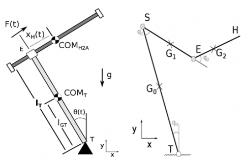
Sitting control results from active contribution (flexor muscles and erector back muscles), passive contribution called also joint resistance (tissues and bones that contribute mechanically to preserve the integrity of the spine) and neuronal contribution (command and sensory) [1, 2]. A person with complete spinal cord injury (SCI) can no longer control the muscles below the level of injury which impairs the ability to maintain a sitting position, particularly when it is disturbed. For the sake of autonomy, patient must then learn new strategies which involves head and upper limbs actions [3]. In order to provide quantified elements to the occupational therapists in monitoring this learning, the joint torques generated (active and passive) by the patients in an attempt to maintain their balance can be considered. Since direct measurement of joint torques is invasive, a so-called “model-based” approach is necessary. The estimation of these joint torques can be performed via inverse dynamics, an approach commonly used in biomechanics, or with the help of particular observers, such as PI-observers, belonging to the class of unknown input observer (UIO) [4]. Few mechanical models of sitting posture exist in the literature, but most of them have limitations and/or are not suitable for people with SCI. Estimating joint torques supposes keeping a model close to reality i.e., without simplifications (such as linearization or neglecting nonlinear terms for example). Models that apply, for example, a linearization around the equilibrium state, as in the study [5, 6, 7] are not adapted because it is an assumption only valid for small movements around this state, whereas it is intended to cope with a model compatible with large movements. Also, models controlled through an active joint located at the lumbosacral joint [8] are not suitable to estimate internal torques for people with SCI, as they generally experience paralysis or paresis of their abdominal and lower back muscles. Indeed, in the absence of voluntary control at the lumbar level, sitting control uses the upper limbs as a compensatory stabilization strategy [9]. A first model allowing to study postural control in sitting position of people with SCI taking into account the contribution of the upper limbs and based on the use of an UIO has been proposed in the study [10]. This model, known as H2AT for «Head-2-Arms-Trunk», was created on the basis of tools developed in the study [11, 12] and is inspired by human movements observed in a clinical setting. The H2AT mechanical model includes two solids: the first rod is the trunk as a classical inverted pendulum and the second rod represents the head and upper limbs sliding at the top of the first solid according to a prismatic joint with a constant angle.
The H2AT model (Figure 1) is based on a mechanical assumption of linear displacement of the center of mass (COM) of the head and upper limbs with respect to the trunk, thereby limiting the inertial effects of rotation of the upper limbs at the shoulder and elbow. This assumption is both important and limiting from an experimental and mechanical point of view, this point was discussed in the study [9]. To address these limitations, an extension of the H2AT model has been introduced in the study [9] through the S3S model, for “Seated-3-Segments”. It consists of a triple inverted pendulum represented in the sagittal plane defined by the trunk, arms and forearms. The S3S model is close to human anatomy compared to the H2AT model, however its development comes at the cost of increased modeling complexity and conditions required for observer synthesis. In the study [13] we show that these conditions are close to the limits of actual solvers [14]. Then, the main problem if we want to enrich this model, for example going from 2D-S3S to 3D-S3S, it is unlikely that a global approach will be compatible with the solvers. To overcome this drawback, an idea is to find a decomposition of the main global problem into smaller subproblems while keeping a good estimation quality [15]. This approach is possible with a cascade of descriptor observers and has been proposed and fully discussed in the study [16], it will be referred to as “decomposed-S3S”. This approach allows to solve locally each observation problem while maintaining a proof of asymptotic convergence of the estimation error, leading to a good trade-off between complexity and estimation quality.
The aim of this paper is to present the decomposed-S3S model, answering the limitations of the previous models, and to study the validity of the approach associating the nonlinear decomposed-S3S model to an UIO through numerical simulations and data-based experiments. This paper is organized as following: the first section is dedicated to the decomposed-S3S model, the second section describes the design of the cascade observers and the final section presents results issued from numerical simulations and data-based tests.
Figure 1. Left: The H2AT model; Right: The S3S model
2.1 The S3S decomposed model
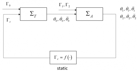
The decomposed-S3S model (Figure 2) was presented in the study [16], only its equations are recalled here. It is a triple inverted pendulum represented in the sagittal plane defined by three blocks in cascade: the trunk " $\mathrm{T}$ ", the upper limbs "A" and a static decoupling term $\Gamma_c=f(\cdot)$. The indices $(0,1$ and 2) correspond to the trunk, arms and forearms respectively. Anatomical data of flexion/extension of the upper limbs [17, 18] are directly issued from anatomical constraints, and they define the compact set of joint variables (in ° and °/s):
Figure 2. The decomposed-S3S model $\left(\Sigma_T\right.$ and $\left.\Sigma_A\right)$
$\Omega_x=\left\{\begin{array}{cc}-20^{\circ} \leq \theta_1-\theta_0-\pi \leq 60^{\circ} & \left\|\dot{\theta}_0\right\| \leq 29^{\circ} / \mathrm{s} \\ -10^{\circ} \leq \theta_2-\theta_1 \leq 45^{\circ} & ,\left\|\dot{1}_1-\dot{\theta}_0\right\| \leq 57^{\circ} / \mathrm{s} \\ & \left\|\dot{\theta}_2-\dot{\theta}_1\right\| \leq 57^{\circ} / \mathrm{s}\end{array}\right\}$ (1)
For each segment: $\Gamma_i$ is the joint torque, $m_i$ the mass, $l_i$ the length, $l_{G_i}$ the length from the origin to the $\mathrm{COM}$ and $I_{G_i}$ the inertial moment at the COM. Inertial and geometric parameters of the model are issued from the regression rules presented in the study [19]. The inertial parameters $p_i i \in\{1$, $2 \ldots 10\}$ and system matrices are fully described in the study $[16]$.
The trunk model $\Sigma_T$ is expressed by the following equation:
$\left[\begin{array}{c}\dot{x}_T \\ \dot{\Omega}_T\end{array}\right]=\left[\begin{array}{cc}A_T\left(\theta_0\right) & B_T \\ 0 & J\end{array}\right]\left[\begin{array}{l}x_T \\ \Omega_T\end{array}\right]$ (2)
With $\Gamma_U=\Gamma_c+\Gamma_0, x_T=\left[\begin{array}{c}\theta_0 \\ \dot{\theta}_0\end{array}\right], \Omega_T=\left[\begin{array}{c}\Gamma_U \\ \Gamma_U\end{array}\right]$ (3)
$\begin{gathered}A_T\left(\theta_0\right)=\left[\begin{array}{cc}1 & 0 \\ 0 & p_1^{-1}\end{array}\right]\left[\begin{array}{cc}0 & 1 \\ p_2 \frac{\sin \left(\theta_0\right)}{\theta_0} & 0\end{array}\right], B_T=\left[\begin{array}{cc}1 & 0 \\ 0 & p_1^{-1}\end{array}\right], \\ J=\left[\begin{array}{ll}0 & 1 \\ 0 & 0\end{array}\right] .\end{gathered}$
The arm model $\Sigma_A$ is expressed by the following equation:
$\begin{aligned} & {\left[\begin{array}{cc}E_A\left(\theta_2\right) & 0 \\ 0 & I\end{array}\right]\left[\begin{array}{c}\dot{x}_A \\ \Omega_A\end{array}\right]=\left[\begin{array}{cc}A_A\left(x_A\right) & B_A \\ 0 & J_2\end{array}\right]\left[\begin{array}{l}x_A \\ \Omega_A\end{array}\right]} \\ & +\left[\begin{array}{c}0 \\ p_6 \sin \left(\theta_1\right) \\ p_7 \sin \left(\theta_2\right) \\ 0\end{array}\right]+\left[\begin{array}{c}0 \\ C\left(\theta_A\right) \\ 0\end{array}\right]\left[\begin{array}{l}\dot{\theta}_0^2 \\ \ddot{\theta}_0\end{array}\right] \\ & y_A=\left[\begin{array}{ll}I_2 & 0\end{array}\right]\left[\begin{array}{c}x_A \\ \Omega_A\end{array}\right]=\theta_A=\left[\begin{array}{l}\theta_1 \\ \theta_2\end{array}\right]\end{aligned}$ (4)
where, $x_A=\left[\begin{array}{l}\theta_A \\ \dot{\theta}_A\end{array}\right]$,
$\theta_A=\left[\begin{array}{l}\theta_1 \\ \theta_2\end{array}\right]$,
$\Omega_A=\left[\begin{array}{llll}\Gamma_1 & \dot{\Gamma}_1 & \Gamma_2 & \dot{\Gamma}_2\end{array}\right]^T$,
$E_a\left(\theta_2\right)=\left[\begin{array}{cc}p_3 & p_4 \cos \left(q_2\right) \\ p_4 \cos \left(q_2\right) & p_5\end{array}\right]$,
$A_a\left(x_A\right)=\left[\begin{array}{cc}0 & p_4 \sin \left(q_2\right) \dot{\theta}_2 \\ -p_4 \sin \left(q_2\right) \dot{\theta}_1 & 0\end{array}\right]$,
$E_A\left(\theta_2\right)=\left[\begin{array}{cc}I & 0 \\ 0 & E_a\left(\theta_2\right)\end{array}\right]$,
$A_A\left(x_A\right)=\left[\begin{array}{cc}0 & I \\ 0 & A_a\left(x_A\right)\end{array}\right]$,
$J_2=\left[\begin{array}{cc}0 & I_2 \\ 0 & 0\end{array}\right]$,
$B_A=\left[\begin{array}{ccc}0 & 0 \\ {\left[\begin{array}{cc}1 & -1 \\ 0 & 1\end{array}\right]} & 0\end{array}\right]$,
$C\left(\theta_A\right)=\left[\begin{array}{cc}p_8 \sin \left(q_1\right) & p_8 \cos \left(q_1\right) \\ p_9 \sin \left(q_1+q_2\right) & p_9 \cos \left(q_1+q_2\right)\end{array}\right]$.
And finally, the coupling term:
$\Gamma_c=\left[\begin{array}{l}-p_{10} \sin \left(q_1\right) \dot{\theta}_1 \\ -p_9 \sin \left(q_1+q_2\right) \dot{\theta}_2 \\ p_{10} \cos \left(q_1\right) \\ p_9 \cos \left(q_1+q_2\right)\end{array}\right]^T\left[\begin{array}{l}\dot{\theta}_1 \\ \dot{\theta}_2 \\ \ddot{\theta}_1 \\ \ddot{\theta}_2\end{array}\right]-\Gamma_1$ (5)
Obviously, such models representing a seated position for SCI people are open-loop unstable. This instability is due to the absence of control at the level of the lumbosacral joint. A stabilizing control law is therefore necessary prior to implement any PI-observer. This control law must also mimic the behavior of a SCI person, who in the absence of voluntary control at the trunk level will use the upper limbs in order to stabilize himself in a sitting position. In this work, the decomposed-S3S was controlled via a control law defined and synthesized in the study [20].
2.2 Cascade observation problem
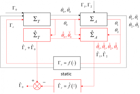
In order to reconstruct unmeasurable joint torques (active at the shoulder and elbow level, passive at the lumber level), a cascade-based approach is used on the decomposed-S3S. Cascade observation has been addressed in the literature by [21, 22]. The idea is to reduce the complexity of the observer design using local observers for each subsystem. The proof of convergence is detailed in the study [16], it uses a classical separation principle. The results lead to two cascaded observers according to the following scheme (Figure 3):
Figure 3. 2 cascade observers for decomposed-S3S model
2.2.1 Takagi-Sugeno formalism
The design of the observers uses a Takagi and Sugeno formalism [23] belonging to the class of quasi-LPV systems, which allows to obtain conditions of convergence of the estimation error. It consists in decomposing a non-linear model into a convex sum of linear sub-models weighted by nonlinear functions that are directly linked to the nonlinearities in the model [15]. Consider a bounded nonlinearity $z_j(\cdot) \in$ $\left[\underline{z}_j, \bar{z}_j\right]$, it exists a convex basis of functions satisfying $\eta_0^j(\cdot) \geq 0, \eta_1^j(\cdot) \geq$0 and $\eta_0^j(\cdot)+\eta_1^j(\cdot)=1$ such that the nonlinearity can be written as $z_j=\underline{z}_j \eta_0^j\left(z_j\right)+\bar{z}_j \eta_1^j\left(z_j\right)$.
$\eta_0^j(\cdot)=\frac{\bar{z}_j-z_j(.)}{\bar{z}_j-\underline{z}_j}, \eta_1^j(\cdot)=1-\eta_0^j(\cdot)$ (6)
An affine nonlinear model in the type control expressed as $E(x) \dot{x}=f(x)+g(x) u, E(x) represents a so-called descriptor form) has a perfect equivalent polytopic model:
$\sum_{i=1}^r v_i(x) E_i \dot{x}=\sum_{i=1}^r v_i(x)\left(A_i x+B_i u\right)$ (7)
$r$ is the number of models, it is in $2^{n l}, n l$ is the number of nonlinearities in the model.
2.2.2 Design of PI-Observers
For the trunk model $\sum_T$ , the PI-observer expression is:
$\left\{\begin{array}{l}{\left[\begin{array}{l}\dot{\hat{x}}_T \\ \dot{\hat{\Omega}}_T\end{array}\right]=\left[\begin{array}{cc}A_T\left(\theta_0\right) & B_T \\ 0 & J\end{array}\right]\left[\begin{array}{l}\hat{x}_T \\ \hat{\Omega}_T\end{array}\right]} \\ +K_T\left(\theta_0\right)\left(y_T-\hat{y}_T\right) \\ \hat{y}_T=C_T \hat{x}_T=\theta_0\end{array}\right.$ (8)
$K_T$ is the observer gain to determine, a simple pole placement has been used. Note that the state has been augmented with a double cascade integrator (hence the name PI-observers). The extended state allows to include the estimation of unmeasurable inputs. For the upper limbs model $\Sigma_A$, the descriptor structure being preserved, the observer has a particular structure [24]. With iE $\{1,2\}, P=\left[\begin{array}{cc}P_1 & 0 \\ P_3 & P_4\end{array}\right], P_1=$ $P_1^T>0$ :
$\begin{aligned} & \sum_{i=1}^2 v_i\left(q_2\right)\left[\begin{array}{cc}E_{A i} & 0 \\ 0 & I\end{array}\right]\left[\begin{array}{l}\dot{\hat{x}}_A \\ \hat{\Omega}_A\end{array}\right]=\left[\begin{array}{cc}A_A\left(\hat{x}_A\right) & B_A \\ 0 & J_2\end{array}\right]\left[\begin{array}{c}\hat{x}_A \\ \hat{\Omega}_A\end{array}\right] \\ & +\left[\left[\begin{array}{c}0 \\ p_6 \sin \left(\theta_1\right) \\ p_7 \sin \left(\theta_2\right) \\ 0\end{array}\right]+\left[\begin{array}{c}0 \\ C\left(\theta_A\right) \\ 0\end{array}\right]\left[\begin{array}{c}\hat{\theta}_0^2 \\ \hat{\hat{\theta}}_0\end{array}\right]\right. \\ & +\left[\sum_{i=1}^2 v_i\left(q_2\right)\left[\begin{array}{cc}E_{A i} & 0 \\ 0 & I\end{array}\right] I\right] P_{(\cdot)}^{-T} \sum_{i=1}^2 v_i\left(q_2\right)\left[\begin{array}{c}K_{1 i}(\cdot) \\ K_{2 i}(\cdot)\end{array}\right]\left(y_A-\hat{y}_A\right) \\ & \end{aligned}$ (9)
$E_{A i}$ are constant matrices. $v_i, w_{i j}$ are the convex weighting functions issued from the TS formalism Eq. (6). They are composed of 3 nonlinearities bounded in the compact set $\Omega_x$ defined in Eq. (1). First, the function $\cos \left(q_2\right) \in[v, 1]$, that can be written with the basis functions $v_1\left(q_2\right)=\frac{1-\cos \left(q_2\right)}{1-v}$ and $v_2\left(q_2\right)=1-v_1\left(q_2\right)$; second the functions $\mathrm{i} \in\{1,2\}$ $\sin \left(q_2\right)\left(\dot{\theta}_i+\dot{\hat{\theta}}_i\right) \in\left[\rho_i, \bar{\rho}_i\right]$ and the basis: $w_{i 1}\left(x_A, \hat{x}_A\right)=$ $\frac{\bar{\rho}_i-\sin \left(q_2\right)\left(\dot{\theta}_i+\dot{\theta}_i\right)}{\bar{\rho}_i-\rho_i}=1-w_{i 2}\left(x_A, \hat{x}_A\right)$
And finally, the stating coupling term $\Gamma_c$ :
$\hat{\Gamma}_c=\left[\begin{array}{l}-p_{10} \sin \left(q_1\right) \hat{\dot{\theta}}_1 \\ -p_9 \sin \left(q_1+q_2\right) \hat{\dot{\theta}}_2 \\ p_{10} \cos \left(q_1\right) \\ p_9 \cos \left(q_1+q_2\right)\end{array}\right]^T\left[\begin{array}{l}\hat{\theta}_1 \\ \hat{\dot{\theta}}_2 \\ \hat{\ddot{\theta}}_1 \\ \hat{\ddot{\theta}}_2\end{array}\right]-\hat{\Gamma}_1$ (10)
First of all, to confirm the validity of the approach, a simulation part is proposed. It allows to access all the simulated variables of the decomposed-S3S (including the torques) and to verify that, on the basis of the only information of the measurable angles, the cascade of observers allows to converge to the unmeasurable variables. In particular, it allows to validate the estimation of the joint torques located at the end of the chain where any uncertainty and modeling error is reflected. Secondly, the cascade of observers is evaluated with real data collected from clinical trials.
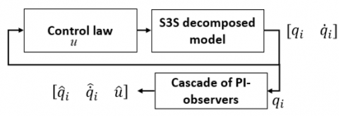
3.1 Simulation test protocol
For simulation purpose, it is mandatory to first stabilize the open-loop. It is done on the decomposed-S3S (Figure 4) using a control law defined in the study [20]. This control law delivers the inputs for the model i.e., the joint torques $u=\Gamma_i$ , i∈{0,1,2}. The cascade PI-observers in Eq. (8), (9) and (10) use as inputs only the measurement of the angles $y^T=\left[\begin{array}{lll}q_0 & q_1 & q_2\end{array}\right]$ to estimate unmeasurable velocities and torques. To test the robustness of the observer, a sinusoidal type signal is added on the joint velocity of the trunk between 2 and 3 seconds. It is compatible (amplitude of accelerations) with real observed disturbances for people with SCI during rehabilitation exercises [25].
Figure 4. Simulation protocol including a stabilizing control law
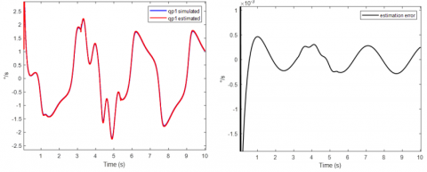
The following figure (Figure 5) give the simulated and estimated shoulder angular velocity $\dot{q}_1, \hat{\dot{q}}_1$ and the estimation error between them.
Figure 5. Angular velocity of the shoulder and estimation error
Observation error is small, around 10-3, which confirms the reliability of the observers. The next step is to assess the validity of the approach using real data collected from clinical trials.
3.2 Data-based experiments
The main objective of this study is to show that it is possible to obtain an estimate of the unmeasured torques, including the passive torque at the lumbar level, from the solution of local problems. In order to specifically solicit the lumbar torque, the long sitting position (straight legs) experiment [26] has been included in the experimental protocol. These experimental tests have received the ethical agreement of Centre de Recherche Interdisciplinaire en réhabilitation du Grand-Montréal (CRIR-1083-0515R). Experimental protocol was fully detailed in the study [9].
26 subjects with SCI (including 14 with an injury located above the T7 vertebra) were involved. Subjects were asked to maintain their seated balance while keeping, if possible, the upper limbs raised. A destabilizing external force applied at the level of the T8 vertebra then disrupted their sitting position. The goal of this force is to challenge sitting stability while ensuring its safety [27]. Two experimental conditions of the lower limbs’ positions have been assessed: 1: straight lower limbs and 2: lower limbs and knee bent at 90°. For each experimental condition, 5 trials have been carried out and measured.
The instructions ask the subject to raise the upper limbs and to maintain this position. 2 to 3 seconds later, a force in the anterior direction is applied to destabilize the subject. The subject must then maintain his sitting balance by adopting compensatory strategies through the action of the upper limbs. Finally, 2 to 3 seconds later and once balanced, the experimenter asks the subject to lower his arms. The cascade PI-observer is used between the moment when the subject is stabilized and the end of stabilization.
Two different subjects have been chosen to illustrate the results: a 32-year-old woman (weight: 55Kg, and height: 163 cm) with SCI at the T6 vertebra for 3 years and a 53-year-old man (weight: 80 Kg, and height: 180 cm) with SCI at the T11 vertebra for 10 years.
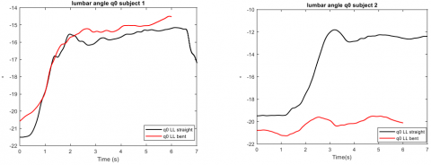
Figure 6 presents lumbar angle $\left(q_0\right)$ for both subjects as a function of the experimental conditions of the lower limbs (straight or bent). The lumbar angle is positive, trunk back from vertical axis, for a bent position of lower limbs and negative; trunk forward from vertical axis, for a straight position of the lower limbs.
Figure 6. Lumbar angle $q_0$ according to lower limbs experimental conditions
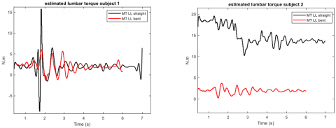
Figure 7. Estimated lumbar torques according to lower limbs experimental conditions
For the same angle, the estimated lumbar torque is given next figure (Figure 7).
The passive torque is on average positive for both subjects. This torque allows to limit the flexion of the trunk. For subject 1, it is on average 5 N.m (resp. 3.25 N.m for subject 2) for bent lower limbs and it is on average 7 N.m (resp. 12 N.m for subject 2) for straight lower limbs. For both subjects the passive torque is higher for extended lower limbs, which is in agreement with the study [26]. In an extended position of the lower limbs, the trunk is located forward of the vertical [9]. The lumbar torque is positive at the beginning of each acquisition, which is consistent from a mechanical point of view because the lumbar angle is negative at the same moment (an articular torque is said to be positive if it rotates a body segment counterclockwise).
The main purpose of this paper is to improve our understanding of sitting stability for SCI persons. In this context, active and passive contributions that control the sitting position despite the absence of motor actions below the injury level have been considered. A bio-inspired model based on movements observed in spinal cord subjects during rehabilitation exercises has been proposed. Through this model, estimation of human joint torques through a cascade PI-observers were designed. The synthesis of these observers uses a quasi-LPV or Takagi-Sugeno formalism and numerical tools for solutions of matrix linear equations (not presented in this paper). The numerical simulation results validate the approach, showing that the cascade PI-observers is able to reconstruct the inputs of the nonlinear S3S model. It is confirmed by clinical results obtained on patients. Compared to the methodologies developed previously in the study [9], the possibility of decomposing the global observation problem into smaller problems allows to consider working with even more complex models, for example a S3S-3D. In addition, this methodology is relevant compared to the inverse dynamics technique commonly used in biomechanics, which consists in deriving experimental position data to recover joint velocity and acceleration of a body segment. The disadvantage of this derivation is that it propagates the estimation errors and can therefore considerably bias the end-of-chain variables that are the joint torques. This approach, which shows its interest, particularly from a methodological point of view, will allow the implementation of more elaborated models. They are useful for improving understanding and carrying out more advanced trials. For example, the experimental recordings show that to counteract the disturbing external force, subjects have adopted compensatory strategies with action of upper limbs outside the sagittal plane. These movements cannot be processed directly with the S3S model and an extension to 3D is in progress.
Modeling and estimating are promising paths to understand situations such as sitting stability of SCI persons. The global approach presented in the study [9] has paved this way, with limitations due to the complexity of the problems to be solved; whose solutions are at the limits of what solvers are able to do today. Going further therefore requires reducing the complexity of the problems to be solved, and a decomposition into local problems has been proposed in the study [16]. A proof of convergence of the global system from local observers showed that this possibility is promising. This approach has been analyzed in this paper both in simulation and in a clinical context. It allows to consider the next step (3D models) with confidence. The goal is to be able, in a long term, to provide relevant data to occupational therapists allowing them to better follow the patient and possibly to see the progress made, for example during a rehabilitation.
[1] Panjabi, M.M. (1992a). The stabilizing system of the spine Part I. Function, dysfunction, adaptation, and enhancement. Journal of Spinal Disorders & Techniques, 5(4): 383-389. https://doi.org/10.1097/00002517-199212000-00001
[2] Panjabi, M.M. (1992b). The Stabilizing System of the Spine. Part II. Neutral Zone and Instability Hypothesis. Journal of Spinal Disorders, 5(4): 390-396. https://doi.org/10.1097/00002517-199212000-00002
[3] Potten, Y.J.M., Seelen, H.A.M., Drukker, J., Reulen, J.P.H., Drost, M.R. (1999). Postural muscle responses in the spinal cord injured persons during forward reaching. Ergonomics, 42(9): 1200-1215. https://doi.org/10.1080/001401399185081
[4] Luenberger, D. (1971). An introduction to observers. IEEE Transactions on automatic control, 16(6): 596-602. https://doi.org/10.1109/TAC.1971.1099826
[5] Masani, K., Popovic, M.R., Nakazawa, K., Kouzaki, M., Nozaki, D. (2003). Importance of Body Sway Velocity.
[6] Qu, X., Nussbaum, M.A., Madigan, M.L. (2007). A balance control model of quiet upright stance based on an optimal control strategy. Journal of Biomechanics, 40(16): 3590-3597. https://doi.org/10.1016/j.jbiomech.2007.06.003
[7] Reeves, N.P., Cholewicki, J., Narendra, K.S. (2009). Effects of reflex delays on postural control during unstable seated balance. Journal of biomechanics, 42(2): 164-170. https://doi.org/10.1016/j.jbiomech.2008.10.016
[8] Tanaka, M.L., Ross, S.D., Nussbaum, M.A. (2010). Mathematical modeling and simulation of seated stability. Journal of biomechanics, 43(5): 906-912. https://doi.org/10.1016/j.jbiomech.2009.11.006
[9] Blandeau, M. (2018). Modélisation et caractérisation de la stabilité en position assise chez les personnes vivant avec une lésion de la moelle épinière (Doctoral dissertation, Université de Valenciennes et du Hainaut-Cambresis).
[10] Blandeau, M., Guerra, T.M., Pudlo, P., Gabrielli, F., Estrada-Manzo, V. (2016). Modelling Seated Postural Stability for Complete Spine Cord Injury. AMSE, Modelling, Measurement & Control, C, 77(2): 40-50.
[11] Grangeon, M., Gagnon, D., Gauthier, C., Jacquemin, G., Masani, K., Popovic, M.R. (2012). Effects of upper limb positions and weight support roles on quasi-static seated postural stability in individuals with spinal cord injury. Gait & posture, 36(3): 572-579. https://doi.org/10.1016/j.gaitpost.2012.05.021
[12] Milosevic, M., Gagnon, D.H., Gourdou, P., Nakazawa, K. (2017). Postural regulatory strategies during quiet sitting are affected in individuals with thoracic spinal cord injury. Gait & posture, 58: 446-452. https://doi.org/10.1016/j.gaitpost.2017.08.032
[13] Blandeau, M., Estrada-Manzo, V., Guerra, T.M., Pudlo, P., Gabrielli, F. (2018). Fuzzy unknown input observer for understanding sitting control of persons living with spinal cord injury. Engineering Applications of Artificial Intelligence, 67: 381-389. https://doi.org/10.1016/j.engappai.2017.09.016
[14] Ortiz, A., Guerra, T.M., Estrada-Manzo, V., Lauber, J. (2021). Choosing an Adequate Convex Structure for Controller and Observer Gains in Takagi-Sugeno Control Systems. IFAC-PapersOnLine, 54(4): 206-211. https://doi.org/10.1016/j.ifacol.2021.10.035
[15] Lendek, Z., Guerra, T.M., Babuska, R., De Schutter, B. (2011). Stability analysis and nonlinear observer design using Takagi-Sugeno fuzzy models, 262. https://doi.org/10.1007/978-3-642-16776-8
[16] Srihi, H., Guerra, T.M., Nguyen, A.T., Pudlo, P., Dequidt, A. (2021). Cascade descriptor observers: Application to understanding sitting control of persons living with spinal cord injury. Frontiers in Control Engineering, 10. https://doi.org/10.3389/fcteg.2021.710271
[17] Kapandji, A.I. (2005a). Anatomie fonctionnelle I: Membres supérieurs. Physiologie de l’appareil locomoteur. 6th edition. Maloine.
[18] Kapandji, A.I. (2005b). Anatomie fonctionnelle III: Tête et rachis. 6th edition. Maloine.
[19] Dumas, R., Cheze, L., Verriest, J.P. (2007). Adjustments to McConville et al. and Young et al. body segment inertial parameters. Journal of biomechanics, 40(3): 543-553. https://doi.org/10.1016/j.jbiomech.2006.02.013
[20] Guerra, T.M., Blandeau, M., Nguyen, A.T., Srihi, H., Dequidt, A. (2020). Stabilizing unstable biomechanical model to understand sitting stability for persons with spinal cord injury. IFAC-PapersOnLine, 53(2): 8001-8006. https://doi.org/10.1016/j.ifacol.2020.12.2225
[21] Lendek, Z., Babuska, R., De Schutter, B. (2008). Stability of cascaded fuzzy systems and observers. IEEE Transactions on Fuzzy Systems, 17(3): 641-653. https://doi.org/10.1109/TFUZZ.2008.924353
[22] Grip, H.F., Saberi, A., Johansen, T.A. (2012). Observers for interconnected nonlinear and linear systems. Automatica, 48(7): 1339-1346. https://doi.org/10.1016/j.automatica.2012.04.008
[23] Takagi, T., Sugeno, M. (1985). Fuzzy identification of systems and its applications to modeling and control. IEEE transactions on systems, man, and cybernetics, 1: 116-132. https://doi.org/10.1109/TSMC.1985.6313399
[24] Guerra, T.M., Estrada-Manzo, V., Lendek, Z. (2015). Observer design for Takagi–Sugeno descriptor models: An LMI approach. Automatica, 52: 154-159. https://doi.org/10.1016/j.automatica.2014.11.008
[25] Bjerkefors, A., Carpenter, M.G., Thorstensson, A. (2007). Dynamic trunk stability is improved in paraplegics following kayak ergometer training. Scandinavian journal of medicine & science in sports, 17(6): 672-679. https://doi.org/10.1111/j.1600-0838.2006.00621.x
[26] Shirado, O., Kawase, M., Minami, A., Strax, T.E. (2004). Quantitative evaluation of long sitting in paraplegic patients with spinal cord injury. Archives of physical medicine and rehabilitation, 85(8): 1251-1256. https://doi.org/10.1016/j.apmr.2003.09.014
[27] John, L.T., Cherian, B., Babu, A. (2010). Postural control and fear of falling in persons with low-level paraplegia. Journal of Rehabilitation Research & Development (JRRD), 47(5): 497-502. https://doi.org/10.1682/JRRD.2009.09.0150