Manas K. Mallick* | Bhanwar S. Choudhary | Gnananandh Budi
OPEN ACCESS
Geostatistics plays an important role for reserve estimation in mining industry. Geostatistical tools became popular because of its high degree of accuracy and time saving process for estimation. The uncertainty of geological deposit can be populated by geo-statistical tools. The limestone ore deposit was studied in this paper. The assay value of individual constituents of limestone ore i.e CaO, SiO2, Al2O3 and Fe2O3 were determined for a block by using Inverse Square Distance Weighting (ISDW) method. The average assay value of those individual constituents were 45.85, 15.94, 1.56 and 0.82 percentage respectively. The assay value of CaO was also estimated by two linear method of estimation i.e ISDW and Ordinary Kriging (OK). The assay value of CaO were determined 45.85 and 44.67 percentage respectively. The assay values were properly validated and concluded accordingly. The application of ISDW and OK were implemented to build the resource model together in order to assess the uncertainty of the deposit. Grade estimation by using different geo-statistical techniques are done by SURPAC mine planning software.
SURPAC software, ordinary kriging, inverse square distance weighting, geostatistics, ore reserve estimation
Mine planning is necessary for determination of total reserve and calculation of average grade value for a particular deposit in order to make it reality. Planning is required for quantifying the resources and bring them by giving some weightage. From the planned data the management can schedule the particular zone where to mine out the mineral at a particular time. Sometime high-grade ore is asked by the management for blending in order to fulfill the demand of market.
A 3-dimensional mining model is developed under a block model and the whole process is known as block modelling. The objective of block modelling is to characterize the whole area into so many blocks but under unidentified mineralization zone [1] Open pit mine planning is done by first generating the solid representative block model from which the average assay value cab be determined. The block model is subdivided into smaller blocks and sub blocks for better valuation [2]. The block model is so framed that the solid ore can be accommodated within that block.
In block model each unit block contains geological attributes i.e. grades of different minerals, specific gravity, partial percentage, rock code, lithology which is predefined before framing a block model. After geological block modelling, the conversion of block economic model by incorporating financial parameters such as mining and process cost, commodity price etc. Block economic model which gives a platform for mine planning and design process [3]. For the estimation process the source of information mostly comes from a restricted number of exploratory boreholes. Due to unavailability of data the whole blocks are not contained the grade value [4]. In resource estimation the value of unsampled blocks are determined from nearby boreholes.
In the field of mine planning and designing several works has been done by various researchers using this software. The mismatch of grade-tonnage and variation in estimation of blocks can be minimized with the help of geo-statistics [5]. Ore body modelling and comparative study of different geo-statistical tools for reserve estimation has been studied [6].
The distance between different sample point to the estimating points are considered in inverse square distance weighting technique in geo-statistical analysis [7]. The assumption is made on the basis of, sampled points have the same distance to the unsampled point will show the equal resemblance [8]. The resemblance of assay value depends on the distance between the two sample points. This method of estimation depends upon the weight of the sample point as well as the distance between the two points to be calculated. The inverse square distance weighting technique is coming under the deterministic method of interpolator [9]. The method of estimation is very simple and easy to implement in mine planning sector.
OK method is a probabilistic method of valuation in order to figure out the uncertainty of ore deposit [10]. Kriging estimator unites the co-variance of different points in a sample and co-variance between the sample location and prediction point [11]. Kriging estimator minimizes the prediction error or error variance. So, the quantity known as mean square prediction error.
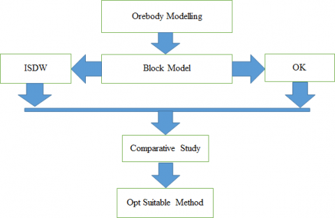
An attempt is made for relative study of linear geo-statistical techniques for resource estimation of a limestone ore deposit in this paper (Figure 1). Both inverse square distance weighting and ordinary kriging estimators are used for assessment of whole ore block after assigning attributes and constraints as well.
Figure 1. Illustration of the application of estimation
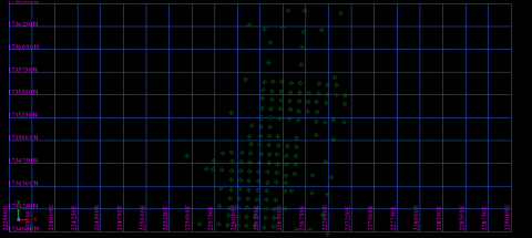
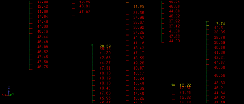
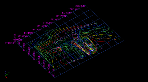
The borehole data of a limestone deposit is used as the main input data to showcase how this software is applied in reserve estimation for both geo-statistical methods. The drill hole database is created and those drill holes are shown in a contour plan (Figure 4). Down the drill holes the assay value of CaO was indicated in order to classify them (i.e. high grade, low grade and waste) along the drill hole depth with different colors (Figure 3). The assay value of every section along the length of the drill hole is shown with unique number for representing the grade of that particular section.
Figure 2. Drillhole layouts
In the process of electronic ore reserve estimation, total 156 numbers of exploratory bore hole data from a limestone ore deposit is used (Figure 2). Geological database is generated by using exploratory bore hole data. The assay values are composited within the interval of 1.5 m down the hole with minimum 75% utilization of sample. Composited assay values are taken for development of geo-statistical model.
Figure 3. Illustration of drill holes labeling
Finally, estimation is done by using both linear geo-statistical techniques for getting the mean assay value of the deposit. The statistical data of limestone ore shows the frequency of population in the data set for initial knowhow about the deposit.
SURPAC software is used for solid ore modelling as well as block modelling in this work. For better grade determination block model is normally developed because the whole focused area is divided into smaller blocks. The smaller blocks are investigated systematically for getting good resource estimation.
Figure 4. Illustration of drill holes in contour plan
2.1 Basic statistics
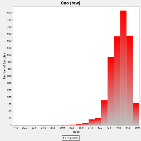
In every 2 m run length down the hole, raw data has been composited. From the composited assay value, a statistical report (Table 1) is generated for analysis purpose. Several frequency of grade values is found from the histogram (Figure 5). The grade values are of negatively skewed.
Table 1. Statistical report of raw data
|
Type |
Value |
|
Number of samples |
3041 |
|
Minimum value |
16.81 |
|
Maximum value |
50.47 |
|
Mean |
45.15 |
|
Median |
45.66 |
|
Geometric mean |
45.03 |
|
Standard Deviation |
2.99 |
|
Variance |
8.96 |
|
Coefficient of variation |
0.06 |
|
Skewness |
-2.26 |
|
Kurtosis |
15.10 |
Figure 5. Histogram of raw data of limestone ore
Twenty numbers of histogram bar are drawn for the frequency analysis of assay value. Statistical analysis is required to provide the idea about the presence of outlier as well as bi-modal distribution in the data set. Outlier is removed from the data set for variogram analysis in order to minimize the error in estimation.
2.2 Solid Ore modelling
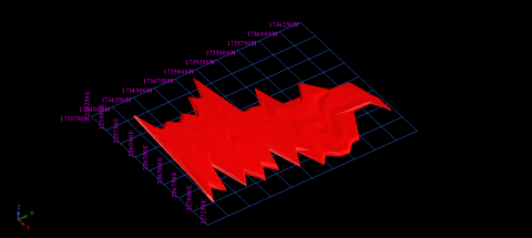
The solid modelling or 3-D modelling is the visualization of the extent of orebody that is captured within the boundary limit (Figure 6). The individual segment of mineralization zone was triangulated in order to form the solid ore body by sectioning followed by digitizing. The segments were undergone different cleaning test (i.e. cross-over, duplicate points, spikes) before forming a solid ore body. After completion of the test, the segments were joined one by one to form a solid ore body. At last, the solid ore body was validated with no error. After validated the ore body model, the area and volume of solid report was obtained which is in Table 2.
Table 2. Object report of solid ore modelling
|
Layer Name: ore.dtm |
|
|
Object: 8 |
|
|
Trisolation: 1 |
|
|
Validated=true |
|
|
Status=solid |
|
|
Trisolation Extents |
|
|
X Minimum: 225394.714 |
X Maximum: 227223.451 |
|
Y Minimum: 1733968.000 |
Y Maximum: 1736168.000 |
|
Z Minimum: 157.183 |
Z Maximum: 253.318 |
|
Surface area: 4544957 |
|
|
Volume: 87622041 |
|
Figure 6. Solid model of ore body
2.3 Block modelling
Block modelling is the basic need for reserve estimation process. For validation of the block model, comparison was made in between volume of block model and volume of solid ore model. For generating a block model different steps which are followed by using SURPAC software.
(a) Creation of empty block model
Block model formation generally involved the block name, its perimeter and size of the block. On the basis of the bench height and width block size of 20 m x 20 m x 10 m and sub block size of 10 m x 10 m x 5 m was used for estimation (Table 3).
Table 3. Summary of block model
|
Type |
Y |
X |
Z |
|
Minimum Coordinate |
1733968 |
225394.714 |
157.183 |
|
Maximum Coordinate |
1736168 |
227234.714 |
257.183 |
|
User Block Size |
20 |
20 |
10 |
|
Minimum Block Size |
20 |
20 |
10 |
|
Total Blocks |
42288 |
||
(b) Adding of attributes
Each block information in the block model were added in the empty blocks by attributes [12]. They included the assay value of each mineral constituents, specific gravity, rock code, partial percentage. Value of attribute can be edited for further modification of estimation during the whole process
(c) Adding of constraints
The selections of blocks are controlled by adding constraints in the block model. The information was retrieved from the block model by selecting the constraint for viewing the model in graphics [13]. One or more spatial objects are logically combined for declaring a constraint. Different logical operators are employed to get the value intersected with in the block model. Finally, the operation is carried out on those chosen blocks [14]. Some of the constraints types used were: block attribute such as the grade, which was used to define the waste, high grade, low grade and medium grade ore using a set cut off value.
(d) Filling the block model by assigned attributes
Some model attribute values were filled directly as background value which will be reflected in the block model directly [15]. The grade value had to be assigned by interpolation method.
2.4 Block grade estimation
Inverse square distance weighting technique and ordinary kriging method were used for calculation of the block value as well as the volume and tonnage.
Inverse square distance weighting technique
Inverse distance weighting is a method which applies a weighting factor that is based on an inverse distance function to each sample with a set of known sample value about the central point of an unknown point of ore block [16]. The weighting factor is the inverse of the distance between each known sample value and the unknown central sample point, raised to the power ‘n’, where n is a positive integer [17].
$Z_{\text {estimated }}=\frac{\sum_{i=1}^{n} \frac{Z_{i}}{d_{i}^{n}}}{\sum_{i=1}^{n} \frac{1}{d_{i}^{n}}}$ (1)
where: Zestimated – Point of sample value to be estimated;
Zi – Known sample value at ith location;
di – Distance between the point of sampled location to the point of sample location to be estimated;
n – Power of the separation distance (d) (in this paper square distance i.e. n=2);
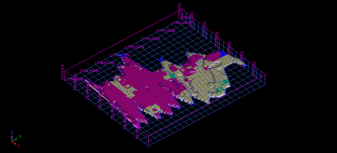
The ore block model having different colors by attribute are shown in (Figure 7). The percentage of CaO value is shown by different colors for each and every block.
Figure 7. Block model of the deposit showing colors by attribute in ISDW method
Figure 8. Block model of the deposit showing colors by attribute in OK method
ordinary kriging
The most frequently used kriging technique is Ordinary Kriging. It is a geo-statistical tool which is defined by the abbreviation BLUE- “best linear unbiased estimator”. It is “best” because the errors in variance can be minimized, “linear” because the estimation values are linear weighted combination of the existing data, and “unbiased” since it attempts to have the error equal to zero [18].
Kriging principle is to estimate values of a delegated variable at a selected location, based on the surrounding existing values [19]. A relevant weighting coefficient is assigned to the selected locations which represents the influence of particular data on the value of the final estimation at the selected grid node [20].
The linear external parameter i.e. Lagrange factor (β) is used to minimize the kriging variance in Ordinary Kriging method. The errors can be minimized by the limiting factor and assessment becomes impractical. The sum of all weights equal to 1, when evaluating the Ordinary Kriging technique [21]. The matrix form of OK equation is given below,
$\left[\begin{array}{cccc}\gamma\left(K_{1}-K_{1}\right) & \gamma\left(K_{1}-K_{2}\right) & \cdots & \gamma\left(K_{1}-K_{n}\right) 1 \\ \gamma\left(K_{2}-K_{1}\right) & \gamma\left(K_{2}-K_{2}\right) & \ldots & \gamma\left(K_{2}-K_{n}\right) & 1 \\ \gamma\left(K_{3}-K_{1}\right) & \gamma\left(K_{3}-K_{2}\right) & \cdots & \gamma\left(K_{3}-K_{n}\right) & 1 \\ \vdots & & & \\ \gamma\left(K_{n}-K_{1}\right) & \gamma\left(K_{n}-K_{2}\right) & \ldots & \gamma\left(K_{n}-K_{n}\right) & 1 \\ 1 & 1 & 1 & 0\end{array}\right] \times\left[\begin{array}{c}\alpha_{1} \\ a_{2} \\ a_{3} \\ \vdots \\ \alpha_{n} \\ \beta\end{array}\right]=\left[\begin{array}{c}\gamma\left(K_{1}-X\right) \\ \gamma\left(K_{2}-X\right) \\ \gamma\left(K_{3}-X\right) \\ \vdots \\ \gamma\left(K_{n}-X\right) \\ 1\end{array}\right]$ (2)
where: $\gamma$– Variogram values,
K1, K2……. Kn-Known sample value at location 1, 2……. n,
X– Estimated new value location,
$\beta$ – Lagrange factor,
α1, α2....... αn-assigned weight values to the data set. The percentage of CaO value is shown by different colors for each and every block which is shown in Figure 8.
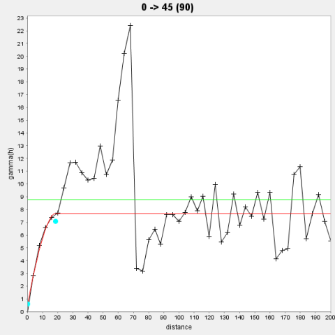
Along with different direction, variogram models are established by using the set of data. From variogram model, the values (nugget, sill and range) are used by Ordinary Kriging method. The grade value of unsampled location are estimated later on by using the calculated variogram model value. Variogram models (Figure 9-10) with azimuth 0° as well as 45° are prepared by using the present case study data. The report of variogram model is given in Table 4.
Figure 9. Illustration of variogram model with azimuth 0°
Figure 10. Illustration of variogram model with azimuth 45°
Table 4. Report of variogram model
|
Serial No. |
Model Type |
Nugget |
Sill |
Range |
|
01 |
Spherical |
1.11 |
6.55 |
16.94 |
|
02 |
Spherical |
1.07 |
6.35 |
15.69 |
Conventional resource estimation was the key process to measure the resource quantitatively. This procedure was the prime estimator and time-consuming process for resource valuation. In order to simplify the estimation process, the application of computer in mine planning and design was involved. In the present study the ore block model was estimated by both Inverse square distance weighting and ordinary kriging methods. The estimated statistical data from both the estimator were related with the basic statistics data. From the comparison it was found that, the inverse square distance weighting method for this resource block got overemphasized. Estimated % of CaO by both ISDW and OK techniques along with the % of CaO in raw data is given below in Table 5.
Table 5. Estimation result of CaO value
|
Statistical parameters |
% CaO in raw data |
% CaO in ISDW |
% CaO in OK |
|
Mean |
45.15 |
45.85 |
44.67 |
|
Variance |
8.96 |
12.64 |
21.28 |
|
Coefficient of variation |
0.06 |
0.08 |
0.10 |
|
Skewness |
-2.26 |
-4.57 |
-8.56 |
The above table shows that, the estimated % of CaO value in Ordinary Kriging (OK) is nearer to the % of CaO value in raw data. The estimated % of CaO values in Inverse Square Distance Weighting (ISDW) overemphasizes the raw value of CaO. The estimated block grade values for different geo-statistical methods are cross checked by creating sections from the bock models. The estimated % of CaO value in Ordinary Kriging and % of CaO value in Inverse Square Distance Weighting are compared with % of CaO values of borehole data for the respective sections. The observation was made that, the % of CaO value in Ordinary Kriging is nearby to the % of CaO value in raw data. In Inverse Distance Weighting technique, the weightage (grade value) between two sample points are taken into consideration and it takes two sample points for calculation. In Kriging method, the weightage (grade value) of multiple points are taken into consideration and calculation is done by using a tedious formula, thereby giving a small average value.
From the study it was revealed that, comparing the grades of CaO for the mentioned block using the two different grade estimation techniques, found that the grades by, Inverse Square Distance Weighting and Ordinary Kriging methods come out to be 45.85% and 44.67% respectively. The total volume for the 3-Dimensional solid ore model is 87622041 m3. The overall surface area of the solid model, i.e. 4544957 m2. Inverse Square Distance Weighting method overemphasizes assay value in comparison to ordinary Kriging.
This work is supported by Department of Mining Engineering, IIT (ISM) Dhanbad for providing us with all the necessary facilities and constant encouragement. We also place on record, our sense of gratitude to one and all who, directly or indirectly, have lent their helping hand in this venture.
[1] Isaaks, E.H., Srivastava, R.M. (1989). An Introduction to Applied Geo-Statistics. Oxford University Press, New York.
[2] Haldar, S.K. (2013). Mineral Exploration- Principles and Practices. Elsevier Publications, 157-182. https://doi.org/10.1016/C2011-0-05550-3
[3] Moharaj, M.C., Wangmo, Y. (2014). Ore body modelling and comparison of different reserve estimation techniques. E-Thesis, National Institute of Technology, Rourkela.
[4] Luo, Z.Q., Liu, X.M., Su, J.H., Wu, Y.B., Liu, W.P. (2007). Deposit 3D modelling and application. Journal of Central South University of Technology, 14: 225-229. https://doi.org/10.1007/s11771-007-0045-9
[5] Stone, J.G., Dunn, P.G., (1994). Ore reserve estimates in the real world. Society of Economic Geology, Publication, 3: 150-154. https://doi.org/10.5382/SP.03
[6] Krige, D.G. (1951). A statistical approach to some basic mine valuation problems on the Witwatersrand. Journal of the Chemical, Metallurgical and Mining Society of South Africa, 52(6): 119-139.
[7] Malvic, T., Balic, D. (2009). Linearity and Lagrange linear multiplicator in the equation of ordinary kriging. NAFTA, 59(1): 31-37.
[8] Malvic, T., Cvetkovic, M., Balic, D. (2008). Geo-Mathematical Dictionary.
[9] Dzimunya, N., Radhe, K., William, C.M. (2018). Design and dimensioning of sublevel stoping for extraction of thin ore (< 12 m) at very deep level: a case study of konkola copper mines (kcm), Zambia. Mathematical Modelling of Engineering Problems, 5(1): 27-32. https://doi.org/10.18280/mmep.050104
[10] Gemcom (Tutorials)- SURPAC software. https://neubrixlaubreak.wixsite.com/knowilulur/single-post/2018/01/22/Gemcom-Surpac-6-4-1-Tutorial, accessed on 12 June 2019.
[11] Roy, D., Butt, S., Frempong, P.A. (2004). Geostatistical resource estimation for the Poura narrow-vein gold deposit. CIM Bulletin, 97(1077): 44-51.
[12] Jayanthu, S., Karthik, G. (2018). Evaluation of stability of cutslopes in open cast metal mines using numerical modelling and field monitoring. Modelling, Measurement and Control C, 79(1): 12-15. https://doi.org/10.18280/mmc_c.790103
[13] Mai, N.L., Bui, X.N. (2016). Application of geo-statistical tools to assess geological uncertainty for Sinquyen Copper mine, Vietnam. Mining Science and Technology, (2): 24-29. https://doi.org/10.17073/2500-0632-2016-2-24-30
[14] Ramani, R.V., Mazumdar, B.K., Samaddar, A.B. (1991). Geostatistics in mining: The current trend. Computers in the mineral Industry, Proceedings of the Indo-Us Seminar, pp. 11-15.
[15] Rao, V.K., Shiva Kumar, T., Sharma, V., Tiwari, P. (2014). Geostatistical modelling and grade estimation of an Iron ore deposit through ordinary kriging A Case Study, NMDC Ltd.
[16] Roy, I., Sarkar, B.C. (2000). Ore body modelling: An integrated geological-geostatistical approach. Department of Applied Geology, IIT (ISM) Dhanbad.
[17] Roy, D., Butt, S.D., Frempong, P.K., Sinha, S.K, Choudhary, B.S., Sharma, R.K. (2017). Review of exploration data with respect to outlier’s experience deposit of NMDC Ltd. Journal of Mines, Metals and Fuels.
[18] Sahoo, M.M., Pal, B.K. (2016). Geological modelling of a deposit and application using SURPAC. National Institute of Technology, Rourkela.
[19] Sarkar, B.C., Roy, I. (2005). A geostatistical approach to resource evaluation of Kala iron Ore Deposit, Sundergarh District, Orissa. Journal of the Geological Society of India, 65: 553-561.
[20] Torabi, A.S., Choudhary, B.S. (2017). Conventional and computer aided ore reserve estimation. International Journal of Engineering Technology Science and Research, 4(12): 896.
[21] Vann, J., Guibal, D. (1998). An overview of nonlinear estimation. In Proceedings of a One-Day Symposium: Beyond Ordinary Kriging, Geostatistical Association of Australia, Perth, Australia, pp. 6-25.