Ashok Misra | Soumyendra Mishra | Abdul Kaffoor Abdul Hakeem | Manoj Kumar Nayak*
OPEN ACCESS
The purpose of the present study is to analyze the flow, heat and mass transfer characteristics in the three dimensional magnetohydrodynamic stretched flow of Cross nanofluids. In the present study, Brownian movement, thermophoresis, thermal and solute convective boundary conditions are considered. With boundary layer approximation and self-similarity transformations, the non dimensional nonlinear governing equations are solved via shooting iteration technique together with 4th order Runge-Kutta integration scheme. The impact of developed physical parameters on velocity, temperature, concentration, surface viscous drag, heat and mass transfer rates has been examined via appropriate graphs and discussions. The numerical results indicate that uplift in the magnetic field strength and Weissenberg number diminishes the axial and transverse velocity fields. Further, the temperature ratio parameter brings about substantial improvement to the temperature and the related layer. The outcomes of the present study provide significant contribution to the controlled fluid motion and regulating the rate of heat transportation from the solid boundary into the boundary layer.
3D stretching sheet, unsteady flow, Brownian motion, thermophoresis, convective boundary conditions
Over a period of fifty years, many noteworthy researchers have put much effort to ensure quality research from both the theoretical as well as experimental fronts. Till date, different researchers have investigated flows of different fluids over surfaces subject to different boundary conditions. In recent times, a novel type of fluid called as nanofluid was introduced by Choi [1] to meet the cooling requirements for production. Nanofluid is a suspension and dispersion of solid nanoparticles (diameter 1–100 nm) in the base fluid. Usually, solid nanoparticles are composed of metals, oxides, carbides or carbon nanotubes while water and organic fluids such as oil, ethanol and ethylene glycol are considered as base fluids. The sizes of nanoparticles are relatively close to the molecules of the base fluid implying stable suspension with little gravitational settling over long time. In contrast to traditional suspensions, nanofluids exhibit high mobility, negligible pressure drop, better suspension, stability, and less mechanical abrasion. In fact, the dispersion of nanoparticles in a base fluid augments the thermal conductivity of the nanofluids which in turn helps the nanofluids acting as cooling agents in numerous industrial manufacturing processes. Subsequently, boundary-layer stretched flow of a nanofluid was investigated by Khan and Pop [2]. Boundary layer convective flow of a nanofluid was studied by Makinde and Aziz [3] and non-orthogonal stagnation point flow of a nanofluid was analyzed by Nadeem et al. [4].
Among many non-Newtonian liquid flow models, the fluid model according to Cross [5] is unique due to its significant properties like yield stress features, flow in regions of both low and high shear rates, finite viscosity and time constant. This model matches the need in engineering and industrial computations [6, 7]. Azam et al. [8] and Khan et al. [9] investigated numerically the flow behavior of Cross nanofluids under various conditions of motion.
Indeed, magnetic nanofluids have received great attention from researchers due to their potential applications in nuclear fusion, bio-medicine, propulsion and control, drug delivery, metallurgy and transformer cooling (Sheikholeslami et al. [10], Nkurikiyimfura et al. [11]). Song et al. [12] investigated the anisotropic thermal conductivity behavior with an advantage of channel cooling. Irreversibility associated with flow in the Sisko nanomaterial was discussed by Khan et al. [13]. Sheikholeslami et al. [14] analyzed the alumina nanofluid MHD flow through a permeable enclosure showing that the Lorentz force boosts the heat conduction. The Hall and Joule heating effects on peristaltic flow were studied by Bhatti and Rashidi [15]. Nayak et al. [16] studied the influence of variable magnetic field and convective boundary condition on a stretched 3D radiative flow of Cu-H2O nanofluid. Nayak [17] investigated MHD flow and heat transfer on a stretched vertical permeable surface and declared the impact of heat generation/absorption, thermal radiation and chemical reaction there.
Despite the wide coverage of the above mentioned literature survey, the transient three dimensional flows and heat transfer behavior of cross nanofluids subject to suction, thermal and solutal convective boundary conditions have not studied yet. Transient flow behavior and impact of thermal and solutal convective boundary conditions on the flow of cross nanofluids over a three dimensional extended surface is the novelty our study. Numerical simulations are performed by using shooting iteration technique together with 4th order Runge-Kutta integration scheme. The numerical solutions are plotted in well structured graphs and discussed appropriately.
In the present problem, section 1 describes the introduction, section 2 deals with the formulation of the problem, section 3 incorporates the numerical procedure, section 4 reveals the results and discussion and finally section 5 imparts the concluding remarks of the study.
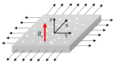
We consider three-dimensional incompressible convective transient flow of magneto Cross nanofluid past a linear permeable stretching sheet. Robust Buongiorno model [18] involving Brownian motion and thermophoresis has been introduced. Fluid is electrically conducting. Magnetic field of strength $B_{0}$ is applied externally along the z-direction. Physical configuration depicting the present model is portrayed in Figure 1.
Figure 1. Flow geometry of the problem (Nayak et al. [17])
The continuity, momentum, energy and nanoparticle concentration equations governing the MHD flow of cross nanofluids are ([2, 3, 7, 8, 18, 19]):
$\frac{\partial u}{\partial x}+\frac{\partial v}{\partial y}+\frac{\partial u}{\partial z}=0$ (1)
$\frac{\partial u}{\partial t}+u \frac{\partial u}{\partial x}+v \frac{\partial u}{\partial y}+w \frac{\partial u}{\partial z}=v \frac{\partial}{\partial z}\left[\frac{\frac{\partial u}{\partial z}}{1+\left(\Gamma \frac{\partial u}{\partial z}\right)^{n}}\right]-\frac{\sigma B_{0}^{2} u}{\rho}$ (2)
$\frac{\partial v}{\partial t}+u \frac{\partial v}{\partial x}+v \frac{\partial v}{\partial y}+w \frac{\partial v}{\partial z}=v \frac{\partial}{\partial z}\left[\frac{\frac{\partial v}{\partial z}}{1+\left(\Gamma \frac{\partial v}{\partial z}\right)^{n}}\right]-\frac{\sigma B_{0}^{2} v}{\rho}$ (3)
$\frac{\partial T}{\partial t}+u \frac{\partial T}{\partial x}+v \frac{\partial T}{\partial y}+w \frac{\partial T}{\partial z}=\alpha \frac{\partial^{2} T}{\partial z^{2}}$
$+\tau\left[D_{B} \frac{\partial T}{\partial z} \frac{\partial C}{\partial z}+\frac{D_{T}}{T_{\infty}}\left(\frac{\partial T}{\partial z}\right)^{2}\right]$ (4)
$\frac{\partial C}{\partial t}+u \frac{\partial C}{\partial x}+v \frac{\partial C}{\partial y}+w \frac{\partial C}{\partial z}=D_{B} \frac{\partial^{2} C}{\partial z^{2}}+\frac{D_{T}}{T_{\infty}} \frac{\partial^{2} T}{\partial z^{2}}$ (5)
The requisite boundary conditions are ([2, 3, 8]):
$\left.\begin{array}{c}u=u_{w}=\frac{a x}{1-c t}, v=v_{w}=\frac{b y}{1-c t}, w=W \\ -k_{f} \frac{\partial T}{\partial z}=h_{f}\left(T_{f}-T\right),-D_{B} \frac{\partial C}{\partial z}=h_{m}\left(C_{f}-C\right) \text { as } z=0 \\ u \rightarrow 0, v \rightarrow 0, \frac{\partial u}{\partial z}=0, T \rightarrow T_{\infty}, C \rightarrow C_{\infty} \text { as } z \rightarrow \infty\end{array}\right\}$ (6)
Here $a>0, b>0$ and $c>0$ are constants having the dimensions $s^{-1}$.
The relevant similarity transformations are:
$\left.\begin{array}{c}u=\frac{a x}{(1-c t)} f^{\prime}(\eta), v=\frac{a x}{(1-c t)} g^{\prime}(\eta), w=-\sqrt{\frac{a v}{(1-c t)}}[f(\eta)+g(\eta)] \\ \frac{T-T_{\infty}}{T_{f}-T_{\infty}}=\theta(\eta), \frac{C-C_{\infty}}{C_{f}-C_{\infty}}=\phi(\eta), \eta=\sqrt{\frac{a}{v(1-c t)}} z\end{array}\right\}$ (7)
Using (6) and (7), (2), (3), (4), and (5) become:
$\left[1+(1-n)\left(W e f^{\prime \prime}\right)^{n}\right] f^{\prime \prime \prime}+(f+g)\left[1+\left(W e f^{\prime \prime}\right)^{n}\right]^{2}$
$-\left\{\left(f^{\prime}\right)^{2}+\lambda\left(f^{\prime}+\frac{\eta}{2} f^{\prime \prime}\right)+M f^{\prime}\right\}\left[1+\left(W e f^{\prime \prime}\right)^{n}\right]^{2}=0$ (8)
$\left[1+(1-n)\left(W e g^{\prime \prime}\right)^{n}\right] g^{\prime \prime \prime}+(f+g)\left[1+\left(W e g^{\prime \prime}\right)^{n}\right]^{2}$
$-\left\{\left(g^{\prime}\right)^{2}+\lambda\left(g^{\prime}+\frac{\eta}{2} g^{\prime \prime}\right)+M g^{\prime}\right\}\left[1+\left(W e g^{\prime \prime}\right)^{n}\right]^{2}=0$ (9)
$\theta^{\prime \prime}+\operatorname{Pr}\left[(f+g) \theta^{\prime}-\frac{\eta}{2} A \theta^{\prime}+N_{b} \theta^{\prime} \phi^{\prime}+N_{t} \theta^{\prime 2}\right]=0$ (10)
$\phi^{\prime \prime}+\left(\frac{N_{t}}{N_{b}}\right) \theta^{\prime \prime}-S c\left[\left(f+g-\frac{1}{2} \lambda \eta\right)\right] \phi^{\prime}=0$ (11)
$\left.\begin{array}{c}f^{\prime}(0)=1, g^{\prime}(0)=1, f(0)+g(0)=S, \\ \theta^{\prime}(0)=-B_{1}[1-\theta(0)], \phi^{\prime}(0)=-B_{2}[1-\phi(0)] \text { at } \eta=0 \\ f^{\prime} \rightarrow 0, g^{\prime} \rightarrow 0, f^{\prime \prime} \rightarrow 0, \theta \rightarrow 0, \phi \rightarrow 0 \text { as } \eta \rightarrow \infty\end{array}\right\}$ (12)
where,
$\left.\begin{array}{c}W e=\frac{\Gamma a \operatorname{Re}^{\frac{1}{2}}}{1-c t}, M=\frac{(1-c t) \sigma B_{0}^{2}}{a \rho}, S=-\frac{W}{\sqrt{a v /(1-c t)}} \\ \operatorname{Pr}=\frac{v}{\alpha}, S c=\frac{v}{D_{B}}, \lambda=\frac{c}{a}, N_{b}=\frac{\tau D_{B}\left(C_{f}-C_{\infty}\right)}{v} \\ N_{t}=\frac{\tau D_{T}\left(T_{f}-T_{\infty}\right)}{v T_{\infty}}, B_{1}=\frac{h_{f} / k_{f}}{\sqrt{a / v(1-c t)}}, B_{2}=\frac{h_{m} / D_{B}}{\sqrt{a / v(1-c t)}}\end{array}\right\}$ (13)
The non-dimensional skin friction, Nussult number and Sherwood number are, respectively
$C_{f x} \operatorname{Re}_{x}^{\frac{1}{2}}=\frac{f^{\prime \prime}(0)}{\left\{1+\left[W e f^{\prime \prime}(0)\right]^{n}\right\}}$ (14)
$C_{f y} \operatorname{Re}_{y}^{\frac{1}{2}}=\frac{g^{\prime \prime}(0)}{\left\{1+\left[\operatorname{Weg}^{\prime \prime}(0)\right]^{n}\right\}}$ (15)
$N u_{x} \operatorname{Re}_{x}^{-\frac{1}{2}}=-\theta^{\prime}(0)$ (16)
$S h_{x} \operatorname{Re}_{x}^{-\frac{1}{2}}=-\phi^{\prime}(0)$ (17)
The numerical solution of the problem is obtained by solving (8)-(11) along with (12) using shooting iteration technique together with 4th order Runge-Kutta integration scheme. In this method we have to choose a suitable finite value of η → ∞ say η∞. Care has been taken to choose the suitable value η∞ for a given set of parameters. The step size is taken as Δη = 0.01. The process is repeated until we get the results correct up to the desired accuracy of 10−7 level, in order to attain the convergence.
A comparison of Nusselt number $\left(N u_{x} \operatorname{Re}_{x}^{-\frac{1}{2}}\right)$ is conducted with the existing study made by Ali [20], Chen [21] and Ishak [22] for different Pr and found to be in excellent agreement (Refer Table 1).
Table 1. Comparison of the present result of Local Nusselt number ($N u_{x} \operatorname{Re}_{x}^{-\frac{1}{2}}$) with Ali [20], Chen [21] and Ishak [22] for different Pr
|
Pr |
Ali [20] |
Chen [21] |
Ishak [22] |
Present Result |
|
0.01 |
- |
0.00991 |
0.0099 |
0.0099113 |
|
0.72 |
0.4617 |
0.46315 |
0.4631 |
0.4631539 |
|
1.0 |
0.5801 |
0.58199 |
0.5820 |
0.5820353 |
The present article examines the flow and heat transfer of unsteady three-dimensional MHD flow of an incompressible Cross nanofluid past a permeable linear stretching sheet. It then added is the Brownian motion, thermophoresis and convective boundary condition to the study. The system of Eqns. (8)-(11) together along with the conditions (12) has been solved numerically via shooting iteration technique together with 4th order Runge-Kutta integration scheme. The general data adopted for the present problem are We = 0.5, n =1, M = 0.5, λ=0.1, Pr=0.3, Sc=1, Nb=0.5, Nt=0.7, B1=B2=10, S=1. A comparative analysis between current study and existing literature shows the accuracy of the present numerical investigation. Going further, we have interpreted the impact of applied physical parameters on the velocity, temperature, nanoparticles concentration, local skin friction, Nusselt number and Sherwood number with far-reaching consequences.
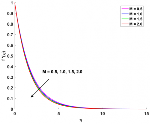
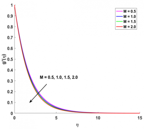
In the analysis, Figures 2 and 3 confirmed that increment in the magnetic field strength (increase in M) produces decelerated flow thereby establishing a thinner VBL along both axial and transverse directions. The decrease of flow axial velocity $f^{\prime}(\eta)$ and transverse velocity $g^{\prime}(\eta)$ is due to the inherent nature of Lorentz force that restrains the motion. Physically, the influence of a transverse magnetic field induces electric current that experiences a force of electromagnetic origin called the Lorentz force. Magnetic parameter is the ratio of electromagnetic force to viscous force. Indeed, higher values of magnetic parameter yielding more Lorentz force which produces more resistance to transport phenomenon. Consequently, the velocity of fluid declines. However, the decrease in axial velocity $f^{\prime}(\eta)$ and transverse velocity $g^{\prime}(\eta)$ is marginal. This is due to the characteristic properties such as definite yield stress, finite viscosity and time constant of the electrically conducting cross nanofluids.
Figure 2. Effect of M on $f^{\prime}(\eta)$
Figure 3. Effect of M on $g^{\prime}(\eta)$
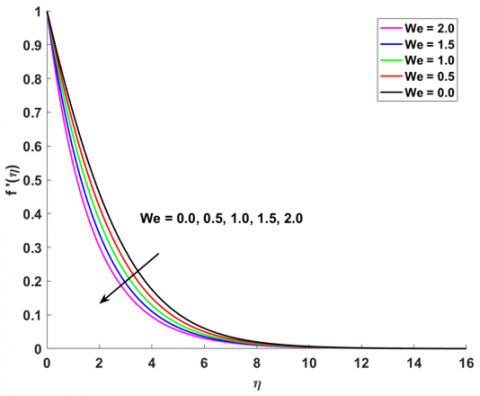
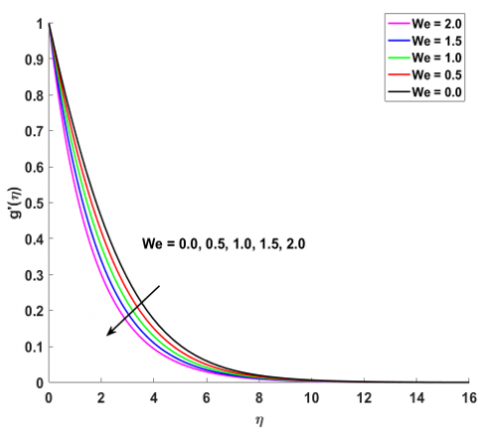
Figure 4. Effect of We on $f^{\prime}(\eta)$
The seemingly well-illustrated axial velocity $f^{\prime}(\eta)$ and transverse velocity $g^{\prime}(\eta)$ profiles for different Weissenberg number We are portrayed in Figures 4 and 5, respectively. Diminution in $f^{\prime}(\eta)$ and $g^{\prime}(\eta)$ and the related layer thickness are due to the increment in We. In case of steady shear, the Weissenberg number is the shear rate times the relaxation time. Weissenberg number improves the thickness of cross nanofluid. As a consequence, velocity of cross nanofluid diminishes due to augmentation of Weissenberg number. Because of this $f^{\prime}(\eta)$ and $g^{\prime}(\eta)$ are strong decreasing functions of We.
Figure 5. Effect of We on $g^{\prime}(\eta)$
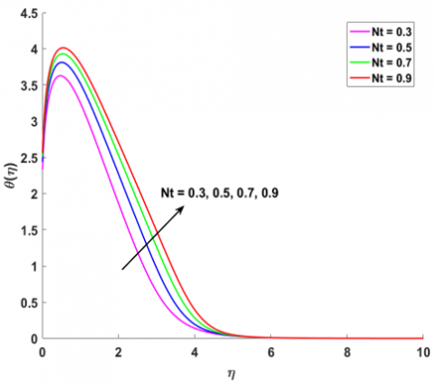
Figure 6. Effect of Nt on $\theta(\eta)$
Figure 7. Effect of Pr on $\theta(\eta)$
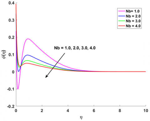
Figure 8. Effect of Nb on $\phi(\eta)$
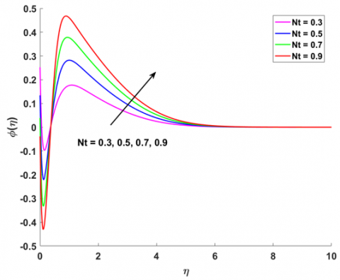
Figure 9. Effect of Nt on $\phi(\eta)$
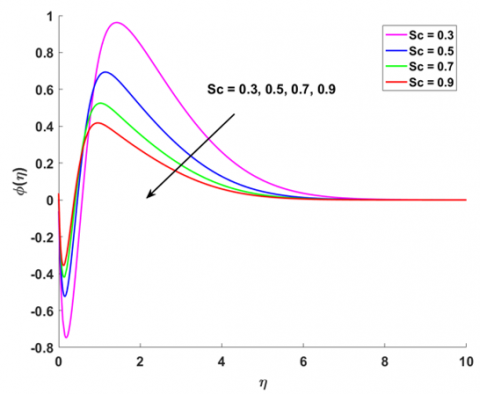
Figure 10. Effect of Sc on $\phi(\eta)$
The characteristics of temperature field $\theta(\eta)$ for thermophoresis parameter Nt and Prandtl number Pr for three-dimensional MHD flow of an incompressible Cross nanofluid are revealed in Figures 6-7. The behavior of $\theta(\eta)$ for different thermophoresis parameter Nt has been demonstrated in Figure 6. The distribution starts with $\theta(\eta)=2.5$ at iη=0 indicating finite temperature distribution. As η increases towards the ambient, θ(η) increases for each Nt and attains its maximum value $\theta_{\max }(\eta)$ at a particular η and then declines sharply and vanishes (θ(η)=0) at η≈6 whatever Nt may be. Larger thermophoresis parameter indicates stronger thermophoretic force. As a result, thermophoretic force drags enormous nanoparticles through greater diffusion from the hot surface towards the ambient thereby increases the fluid temperature within the few layers boundary layer region. This may cause to a change in the structure of thermal boundary layer. Why is there a peak $\theta_{\max }(\eta)$? This is because the temperature of the fluid contiguous to the stretched sheet exceeds the temperature of the ambient fluid.
Higher Prandtl cross nanofluids (represented by high Prandtl number Pr) contributes to the diminishing temperature profiles $\theta(\eta)$ and the related layer thickness as shown in Figure 7. This is because higher Prandtl fluids implicating fluids with lower thermal diffusivity. Therefore, less heat would propagate through such fluids thereby leading to lower temperature. This may also change the structure of thermal boundary layer.
As far as the behavior of nanoparticles concentration $\varphi(\eta)$ is concerned, Figures 8-10 represent $\varphi(\eta)$ profiles in relation to the Brownian motion parameter Nb, thermophoresis parameter Nt and Schmidt parameter Sc for three-dimensional MHD flow of an incompressible Cross nanofluid. The $\varphi(\eta)$ profiles for different Brownian motion parameter Nb are depicted in Figure 8. Increment in Nb decreases the nanoparticles concentration $\varphi(\eta)$ leading to shrinkage of CBL. Physically, the Brownian motion makes the particles to move in opposite direction of the concentration gradient and make the nanofluid more homogenous. Such force leads to low concentration gradient and therefore lesser nanoparticle concentration distribution. However, the profiles of $\varphi(\eta)$ in response to Nt exhibit opposite trend compared to that of Nb (See Figure 9). From physics point of view, larger thermophoresis parameter implicates stronger thermophoretic force. Because of stronger thermophoretic force avalanche of fluid particles are pulled away from hot surface to the cold region and contribute to the enhancement of nanoparticle concentrations. Here, the only difference between the two profiles is that the variation of $\varphi(\eta)$ due to Nt provide more intensification compared to the variation due to Nb. Increase in Schmidt number Sc resulting in diminishing of $\varphi(\eta)$ leading to decreased CBLT (See Figure10). Schmidt number is related with Brownian movement. A rise in Schmidt number prompts poor Brownian movement which in turn yields a decay of nanoparticle concentrations. In other words, fluids with larger Schmidt number indicating more molecular diffusivity makes nanoparticles concentration decline. Why is there a peak $\phi_{\max }(\eta)$? This is because at certain Sc, due to fixed DB nanoparticle concentrations contiguous to the stretched sheet exceed that of the ambient fluid.
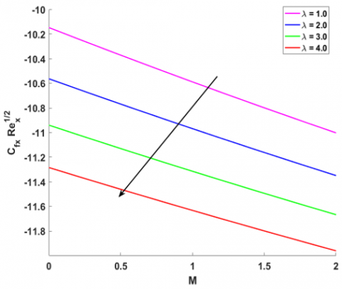
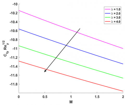
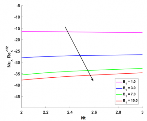
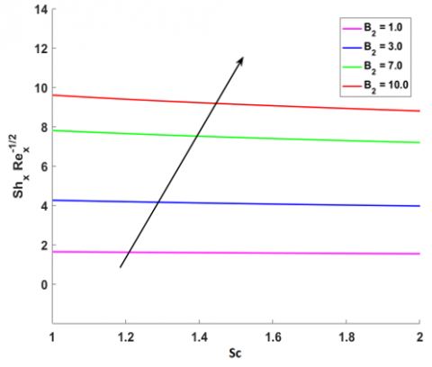
Moreover, Figures 11-14 convey about the behavior of axial skin friction coefficient $C_{f x} R e_{x}^{\frac{1}{2}}$, transverse skin friction coefficient $C_{f y} R e_{y}^{\frac{1}{2}}$, Nusselt number $N u_{x} R e_{x}^{-\frac{1}{2}}$ and Sherwood number $S h_{x} R e_{x}^{-\frac{1}{2}}$ respectively for three-dimensional MHD flow of an incompressible Cross nanofluid. The variation of $C_{f x} R e_{x}^{\frac{1}{2}}$ and $C_{f y} R e_{y}^{\frac{1}{2}}$ representing axial and transverse wall shear stress for various unsteadiness parameter λ against M exhibiting a similar trend as reflected from the Figures 11 and 12 respectively. In both profiles the axial as well as transverse viscous drag of cross nanofluids thrives due to increase in λ. Finally, the variation of Nusselt number $N u_{x} R e_{x}^{-\frac{1}{2}}$ for different thermal convective parameter B1 is shown in Figure 13. Here we may declare that $N u_{x} R e_{x}^{-\frac{1}{2}}$ profiles decline due to increase in B1. In other words, more convective heating leads to undermine the heat transfer rate from the 3D stretched sheet. By convective boundary condition we mean that the sheet surface is heated by a hot fluid through convection with uniform temperature Tf and the convective heat transfer coefficient hf. This implicates that convective heating leads to the augmentation of non-dimensional fluid temperature. The variation in Sherwood number $S h_{x} R e_{x}^{-\frac{1}{2}}$ for mass convective parameter B2 is depicted in Figure 14. It is well-understood from this figure that $S h_{x} R e_{x}^{-\frac{1}{2}}$ thrives due to uplift in B2. This implicates that the mass transfer rate flourishes for improvement in B2.
Figure 11. Effect of λ against M on $C_{f x} \operatorname{Re}_{x}^{\frac{1}{2}}$
Figure 12. Effect of λ against M on $C_{y} \mathrm{Re}_{y}^{\frac{1}{2}}$
Figure 13. Effect of B1 against Nt on $N u_{x} R e_{x}^{-\frac{1}{2}}$
Figure 14. Effect of B2 against Nt on $S h_{x} R e_{x}^{-\frac{1}{2}}$
The present study focuses on the behavior of transient flow of cross nanofluids past a permeable 3D linear stretching sheet. The major important outcomes are:
Increment in magnetic field strength (increase in M) is the cause for the decelerated flow and reduction in the related BLT along both axial and transverse directions.
Diminution in axial velocity $f^{\prime}(\eta)$ and transverse velocity $g^{\prime}(\eta)$ and the related layer thickness are due to uplift in We.
Elevated temperature is the result due to rise in Nt while its depreciation is attained in response to augmented Pr resulting in expanded TBL.
Nanoparticles concentration belittles due to increment in Nb, Nt and Sc thereby contracts the CBL.
Both $C_{f x} R e_{x}^{\frac{1}{2}}$ and $C_{y} R e_{y}^{\frac{1}{2}}$ diminish for rise in λ, $N u_{x} R e_{x}^{-\frac{1}{2}}$ decays for increment in B1 and $S h_{x} R e_{x}^{-\frac{1}{2}}$ ups due to increase in B2.
The present study can be extended by introducing the impact of Thompson and Troian slip and non uniform heat source and sink subject to Darcy Forchheimer flow of micropolar Cross nanofluids.
|
Brownian diffusion coefficient |
$D_{B}\left(m^{2} s^{-1}\right):\left[L^{2} T^{-1}\right]$ |
|
Brownian motion parameter |
$N_{b}=\frac{\tau D_{B}\left(C_{f}-C_{\infty}\right)}{v}$ |
|
Concentration boundary layer |
CBL |
|
Convective heat transfer coefficient |
$h_{f}\left(W m^{-2} K^{-1}\right):\left[M T^{-3} K^{-1}\right]$ |
|
Density of fluid |
$\rho\left(\operatorname{kg} m^{-3}\right):\left[M L^{-3}\right]$ |
|
Eckert number |
$E_{c}=\frac{u_{w}^{2}}{c_{p}\left(T_{f}-T_{\infty}\right)}$ |
|
Fluid velocity components |
$(u, v, w):\left(m s^{-1}, m s^{-1}, m s^{-1}\right):$ $\left(\left[L T^{-1}\right],\left[L T^{-1}\right],\left[L T^{-1}\right]\right)$ |
|
Hartmann number |
$M=\frac{(1-c t) \sigma B_{0}^{2}}{a \rho}$ |
|
Heat capacity ratio |
$\tau=\left(\rho C_{p}\right)_{p} /\left(\rho C_{p}\right)_{f}$ |
|
Heat transfer rate |
HTR |
|
Kinematic viscosity of fluid |
$v:\left(m^{2} s^{-1}\right):\left[L^{2} T^{-1}\right]$ |
|
Local axial skin friction coefficient |
$C_{f i} \operatorname{Re}_{x}^{\frac{1}{2}}$ |
|
Local Nusselt number |
$N u_{x} \operatorname{Re}_{x}^{-\frac{1}{2}}$ |
|
Local Sherwood number |
$S h_{x} \operatorname{Re}_{x}^{-\frac{1}{2}}$ |
|
Local transverse skin friction coefficient |
$C_{f y} \operatorname{Re}_{y}^{\frac{1}{2}}$ |
|
Local Weissenberg number |
$W e=\frac{\Gamma a \operatorname{Re}^{\frac{1}{2}}}{1-c t}$ |
|
Magnetohydrodynamics |
MHD |
|
Mass transfer rate |
MTR |
|
Nanoparticles concentration of the ambient fluid |
$C_{\infty}:\left(k g m^{-2}\right):\left[M L^{-2}\right]$ |
|
Nanoparticles concentration of convective mass transfer |
$C_{f}:\left(k g m^{-2}\right):\left[M L^{-2}\right]$ |
|
Nanoparticles concentration of the fluid |
$C:\left(k g m^{-2}\right):\left[M L^{-2}\right]$ |
|
Prandtl number |
$\operatorname{Pr}=\frac{v}{\alpha}$ |
|
Reynolds number |
$\mathrm{Re}=\frac{u_{w} x}{v}$ |
|
Schmidt number |
$S c=\frac{v}{D_{B}}$ |
|
Solute convective number |
$B_{2}=\frac{h_{m} / D_{B}}{\sqrt{a / v(1-c t)}}$ |
|
Specific heat capacity of fluid |
$c_{p}:\left(J k g^{-1} K^{-1}\right):\left[L^{2} \theta^{-1} T^{-2}\right]$ |
|
Strength of uniform magnetic field |
$B_{0}:\left(N m^{-1} A^{-1}\right):\left[M T^{-2} A^{-1}\right]$ |
|
Suction parameter |
$S=-\frac{W}{\sqrt{a v /(1-c t)}}$ |
|
Temperature of the ambient fluid |
$T_{\infty}:(K):[\theta]$ |
|
Temperature of the convective heat transfer |
$T_{f}:(K):[\theta]$ |
|
Temperature of the fluid |
$T:(K):[\theta]$ |
|
Thermal boundary layer |
TBL |
|
Thermal conductivity |
TC |
|
Thermal conductivity |
$k_{f}:\left(W m^{-1} K^{-1}\right):\left[M L T^{-3} K^{-1}\right]$ |
|
Thermal convective number |
$B_{1}=\frac{h_{f} / k_{f}}{\sqrt{a / v(1-c t)}}$ |
|
Thermal diffusivity |
$\alpha:\left(m^{2} s^{-1}\right):\left[L^{2} T^{-1}\right]$ |
|
Thermophoresis parameter |
$N_{t}=\frac{\tau D_{T}\left(T_{f}-T_{\infty}\right)}{v T_{\infty}}$ |
|
Thermophoretic diffusion coefficient |
$D_{T}:\left(m^{2} s^{-1}\right):\left[L^{2} T^{-1}\right]$ |
|
Velocity boundary layer |
VBL |
|
Subscripts |
|
|
f |
fluid |
|
w |
quantities at wall |
|
∞ |
quantities at free stream |
[1] Choi, S.U.S. (1995). Enhancing thermal conductivity of fluids with nanoparticles. Conference: 1995 International mechanical engineering congress and exhibition, San Francisco, CA (United States), 12-17 Nov 1995; Other Information: PBD: Oct 1995, 231: 99-106.
[2] Khan, W., Pop, I. (2010). Boundary-layer flow of a nanofluid past a stretching sheet. Int. J. Heat Mass Transfer, 53(11-12): 2477-2483. https://doi.org/10.1016/j.ijheatmasstransfer.2010.01.032
[3] Makinde, O., Aziz, A. (2011). Boundary layer flow of a nanofluid past a stretching sheet with a convective boundary condition. International Journal of Thermal Sciences, 50(7): 1326-1332. https://doi.org/10.1016/j.ijthermalsci.2011.02.019
[4] Nadeem, S., Mehmood, R., Akbar, N.S. (2013). Non-orthogonal stagnation point flow of a nano non-Newtonian fluid towards a stretching surface with heat transfer, Int. J. Heat Mass Transfer, 57(2): 679-689. https://doi.org/10.1016/j.ijheatmasstransfer.2012.10.019
[5] Cross, M.M. (1965). Rheology of non-Newtonian fluids: A new flow equation for pseudoplastic systems. J. Colloid Sci., 20(5): 417-437. https://doi.org/10.1016/0095-8522(65)90022-X
[6] Khan, M., Manzur, M., Rahman, M.U. (2016). Boundary layer flow and heat transfer of Cross fluid over a stretching sheet. Thermal Science 23(1). https://doi.org/10.2298/TSCI160919111K
[7] Azam, M., Shakoor, A., Rasool, H.F., Khan, M. (2019). Numerical simulation for solar energy aspects on unsteady convective flow of MHD Cross nanofluid: A revised approach. Int. J. Heat. Mass Transf., 131: 495-505. https://doi.org/10.1016/j.ijheatmasstransfer.2018.11.022
[8] Khan, M., Hayat, T., Khan, M.I., Alsaedi, A. (2018). Activation energy impact in nonlinear radiative stagnation point flow of Cross nanofluid. Int. J. Heat. Mass Transf., 91: 216-224. https://doi.org/10.1016/j.icheatmasstransfer.2017.11.001
[9] Khan, M., Manzur, M., Rahman, M.U. (2017). On axisymmetric flow and heat transfer of Cross fluid over a radially stretching sheet. Results Phys., 7: 3767-3772. https://doi.org/10.1016/j.rinp.2017.08.039
[10] Sheikholeslami, M., Sadoughi, M. (2017). Mesoscopic method for MHD nanofluid flow inside a porous cavity considering various shapes of nanoparticles. Int. J. Heat Mass Transf., 113: 106-114. https://doi.org/10.1016/j.ijheatmasstransfer.2017.05.054
[11] Nkurikiyimfura, I., Wang, Y., Pan, Z. (2013). Heat transfer enhancement by magnetic nanofluids—a review. Renew. Sustain. Energy Rev., 21: 548-561. https://doi.org/10.1016/j.rser.2012.12.039
[12] Song, D., Jing, D., Luo, B., Geng, J., Ren, Y. (2015). Modeling of anisotropic flow and thermodynamic properties of magnetic nanofluids induced by external magnetic field with varied imposing directions. J. Appl. Phys., 118(4): 45101. https://doi.org/10.1063/1.4927043
[13] Khan, M.I., Hayat, T., Qayyum, S., Khan, M.I., Alsaedi, A. (2018). Entropy generation (irreversibility) associated with flow and heat transport mechanism in Sisko nanomaterial. Phys. Lett. A, 382(34): 2343-2353. https://doi.org/10.1016/j.physleta.2018.05.047
[14] Sheikholeslami, M., Shehzad, S.A., Li, Z., Shafee, A. (2018). Numerical modeling for alumina nanofluid magnetohydrodynamic convective heat transfer in a permeable medium using Darcy law. Int. J. Heat Mass Transf., 127: 614-622. https://doi.org/10.1016/j.ijheatmasstransfer.2018.07.013
[15] Bhatti, M.M., Rashidi, M.M. (2017). Study of heat and mass transfer with Joule heating on magnetohydrodynamic (MHD) peristaltic blood flow under the influence of Hall effect. Propulsion Power Res., 6(3): 177-185. https://doi.org/10.1016/j.jppr.2017.07.006
[16] Nayak, M.K., Shaw, S., Chamkha, A.J. (2018). Impact of variable magnetic field and convective boundary condition on a stretched 3D radiative flow of Cu-H2O nanofluid. Modelling, Measurement, Control B, 86(3): 786-798.
[17] Nayak, M.K. (2016). Steady MHD flow and heat transfer on a stretched vertical permeable surface in presence of heat generation/absorption, thermal radiation and chemical reaction. Modelling, Measurement and Control B, 85(1): 91-104.
[18] Buongiorno, J. (2006). Convective transport in nanofluids. ASME J. Heat Transf., 128(3): 240-250. https://doi.org/10.1115/1.2150834
[19] Nayak, M.K., Akbar, N.S., Pandey, V.S., Khan, Z.H., Tripathi, D. (2017). 3D free convective MHD flow of nanofluid over permeable linear stretching sheet with thermal radiation. Powder Technol., 315: 205-215. https://doi.org/10.1016/j.powtec.2017.04.017
[20] Ali, M.E. (1994). Heat transfer characteristics of a continuous stretching surface. Heat Mass Transf., 29: 227-234. https://doi.org/10.1007/BF01539754
[21] Chen, C.H. (1998). Laminar mixed convection adjacent to vertical continuously stretching sheets. Heat Mass Transf., 33: 471-476. https://doi.org/10.1007/s002310050217
[22] Ishak, A. (2010). Thermal boundary layer flow over a stretching sheet in a micropolar fluid with radiation effect. Meccanica, 45: 367-373. https://doi.org/10.1007/s11012-009-9257-4